The present example considers a time domain reflectometry (TDR) application.
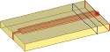
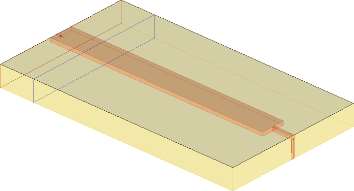
Strip-line structure.
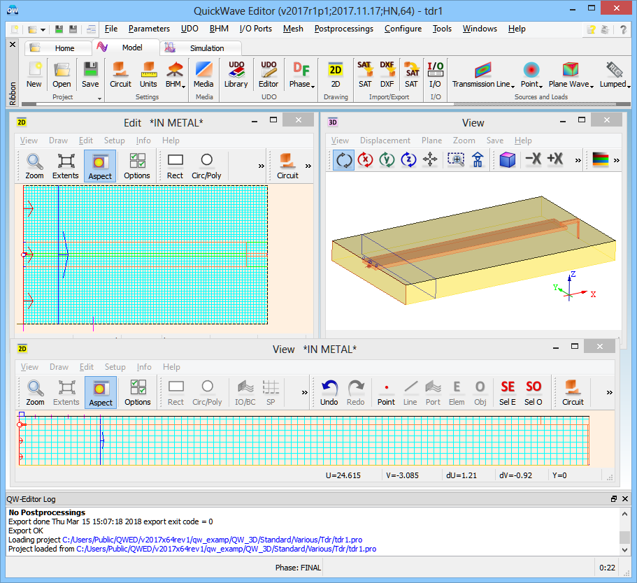
Strip-line structure project in QW-Editor.
TDR-like signals can be extracted directly from QuickWave simulations. In the present case, simulation models contains a strip-line structure and we are considering a lower half of the structure assuming a magnetic symmetry plane. Substrate is a 6 mm thick teflon. The input strip is 1 mm thick, 3.5 mm wide, and 32 mm long. It is terminated by a grounded strip of width 0.5 mm. During the simulation the structure will be excited by a step pulse and we will be considering Ez and Hy fields below the strip, at the point situated 3.36 mm from the input and thus 28.64 mm from the end of the wide strip.
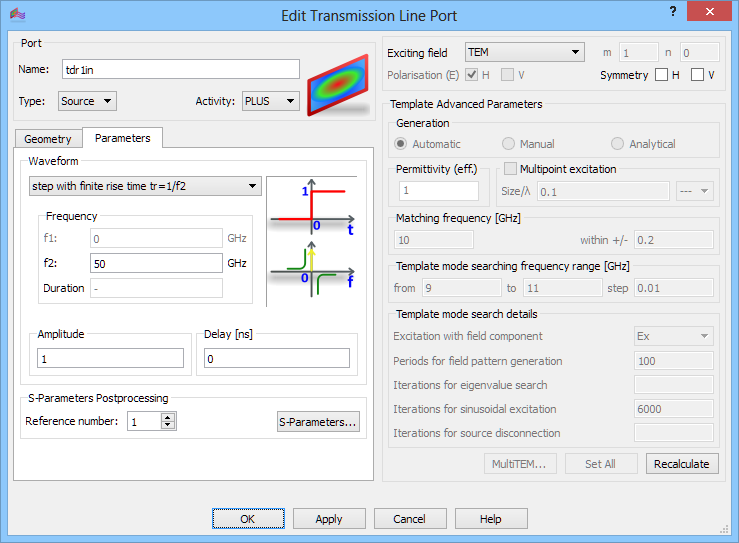
The excitation is a pulse waveform: step with finite rise time dt=1/f2 with f2=50 GHz. Let us justify this choice. In the considered project we use the cell size of 0.4 mm. For correct FDTD analysis the cell size should not be bigger than 0.1 of the wavelength. At 50 GHz the wavelength is 6 mm in air and about 4.2 mm in teflon. Thus with this FDTD mesh we should avoid exciting the circuit at the frequencies significantly higher than 50 GHz. It can be done by introducing a finite rise-time of the pulse.
Excitation settings for transmission line port.
We run the simulation and observe the instantaneous fields distribution in time at a certain point:
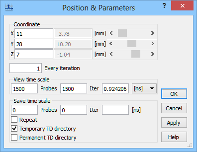
Observation point position dialogue.
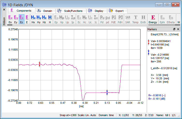
Initially the signal is close to 0. Then when the pulse slope reaches the field testing point, it rises to the incident wave level. The incident wave level is maintained until the wave reflected from the end of the wide line reaches back the field testing point. The narrow line is inductive and thus the reflection coefficient is initially positive (causing that the E-field is amplified). However, since the narrow line is finally short-circuited, the steady state solution must bring reflection coefficient to the value of R=-1 and the field value to 0. The function TDR allows to read the reflection coefficient at any point in time. The reflection coefficient is presented as R=... in linear and dB scale after we place the first (blue) cursor at the point of measurement and the second (red) cursor at the level of the incident wave.
Ez field component versus time in a certain point in space.
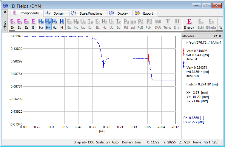
Hy field component versus time in a certain point in space.
The dual behaviour of the magnetic field variations can be observed. Moreover, in this case we would like to illustrate the possibility of measuring the distance between the field testing point and the discontinuity. We set the cursors at the beginning of the first pulse rise and the time point when the wave reflected from the discontinuity starts to perturb the waveform. We read that the time difference between these two points is 0.274 ns. After multiplying this value by the speed of the wave in teflon we obtain 57.68 mm. The distance to the discontinuity should be equal to half of that, i.e., 28.84 mm. In fact, we know that that distance is 32-3.36=28.64 mm. Thus in our virtual TDR experiment we are able to locate both the position of the discontinuity and its character (short circuited inductance).
Time dependent Ez and Hy field components distribution.