2       Interactive operation

For practical application of QW-BHM with its complex and interrelated regimes, we recommend running it in the batch mode described in Batch operation. However, we believe that it is worthwhile to analyse a few examples in an interactive way, so as to gain better understanding of the consecutive BHM steps and to develop confidence in the tool. Moreover, when approaching new scenarios or new thermally-media, the user may wish to perform a short manually-controlled simulation first, to estimate the rate of change of media parameters during the heating and hence to set reasonable defaults for Tasker times in File-Export Options-Allow BHM-Details... dialogue of QW-Editor.

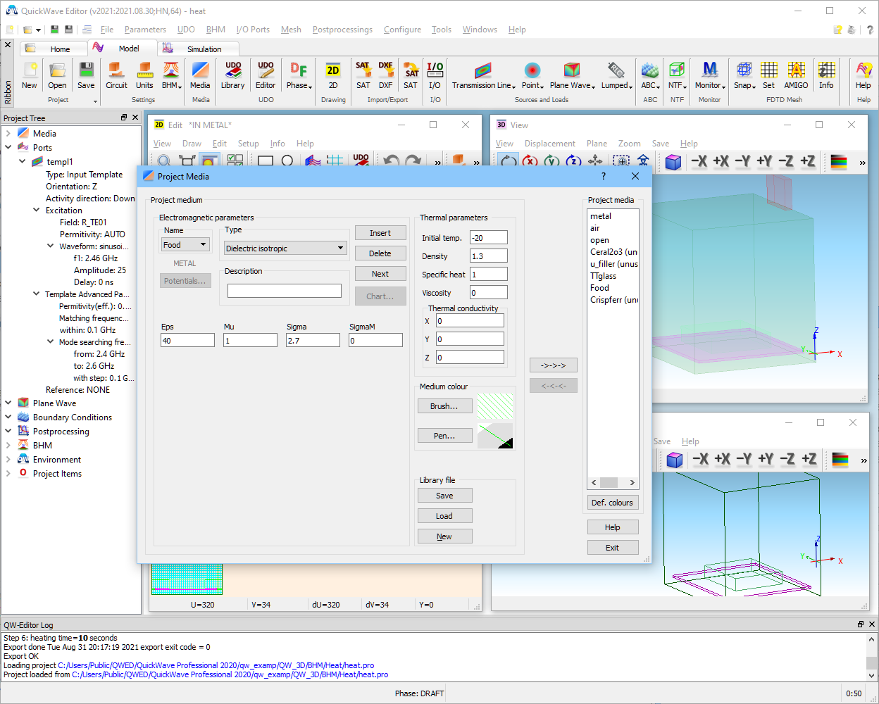
Fig. 2-1 A view of heat.pro example in QW-Editor, with open media dialogue and Heating details dialogue.

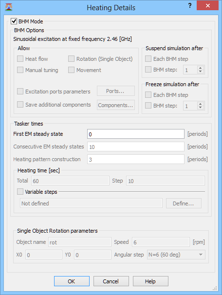
We shall refer to ..BHM\Heat\heat.pro example. This was the first example created for QW-BHM, its early versions, where complicated automatic tasker files were not generated by QW-Editor. The generation of automatic tasker files can be suppressed by forcing the First EM steady state field to 0 periods in the File-Export Options-Allow BHM-Details... dialogue. This is done in heat.pro example, as shown in Fig. 2-1. The remaining Tasker times become irrelevant. The options of heat flow and rotation are not checked, to run the simplest of the BHM modes with media parameters variation only.

It contains a load medium called food, and thus food.pmo file should be available in the project directory for reasonable QW-BHM operation. Two sample files are shown below:

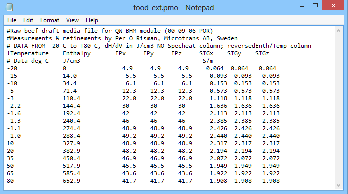
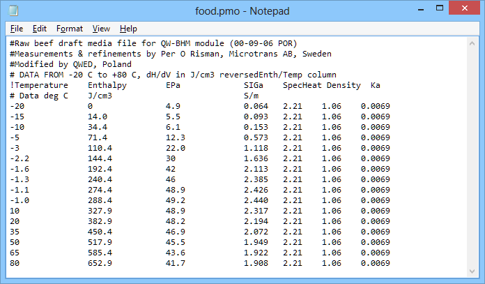
Fig. 2-2 The contents of food.pmo file.

The files contain temperature data and 2.45 GHz permittivity data for raw beef as a function of enthalpy density. The data has been prepared by Per O. Risman, Microtrans AB, Sweden, using various sources (for enthalpy e.g. Rha & Riedel, for permittivity raw and published as well as unpublished own data from SIK). The food_ext.pmo file shows the way of introducing anisotropic parameters, while food.pmo additionally includes thermal parameters needed for heat flow analysis (see Usage of the QW-HFM module).

The top three lines of the file (starting with #) are comments. Then there is a header line (starting with !). The header shows which quantities / parameters are listed in corresponding tables. One more comment line reminds of the units assumed in QW-BHM.

QW-BHM recognises the following keywords, and assumes the following units:

Note: additional requirements for availability of certain columns for QW-HFM (Heat Flow Module) are given in Defining of the media properties.

Among the above keywords, those terminating with “a” (EPa, MUa, SIGa, MSIGa, Ka) are used to set all three directional components of respective tensors for isotropic media.

The user is kindly asked to execute caution when preparing new *.pmo files. Incorrect material data will compromise simulation results, and may even confuse the software! QW-BHM detects a number of most dangerous instances of errors in *.pmo files and, if detected, terminates the simulation:

- illegal keyword (not listed in the table above),

- neither Temperature nor Enthalpy keywords encountered in header,

- number of numerical entries in one of the rows different from the number of keywords,

- error in reading a number (i.e., encountering not a number entry where number is expected).

After the initial header and comments, the file contains eight columns. Note that it describes the variation of enthalpy, permittivity, and conductivity versus temperature, in the temperature range between -20°C and 80°C. If more than 652.9 J/cm³ is absorbed, the temperature and media parameters will remain constant (and equal to those at 652.9 J/cm³). All the remaining parameters of food (not listed in the file – i.e., permeability, magnetic loss, and density) will be constant during the simulation (and equal to those set in QW-Editor, Fig. 2-1).

Before running the analysis, please consult the settings of media parameters in QW-Editor. Default parameters of food are e_r=40, s =2.7 S/m.

Initial temperature of food has been set at -20°C while of all other media in the environment at +20°C. This means that initial enthalpy is zero for food (as taken from the file), as well as for all other media (which have no *.pmo files, and zero is a default). If we modify the initial temperature of food to -15°C, its initial enthalpy will be 14 J/cm³.

Start the QW-Simulator in the usual way (pressing  in QW-Editor). It may be interesting to consult the TestMesh display ( button in Mesh tab). Clicking the Media button in Info tab enables viewing the current values of media parameters (also accessible via Mesh-Media). Note that for food permittivity and conductivity are different from the default settings of QW‑Editor, and equal to the settings of the food.pmo file at initial enthalpy (Eps=4.9, Sigma=0.064 S/m). Other food parameters (permeability, magnetic loss, density) have not been listed in food.pmo and hence remain equal to the settings of QW‑Editor.

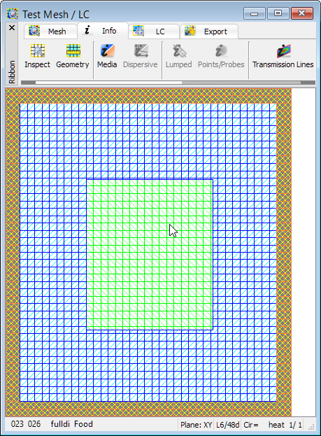
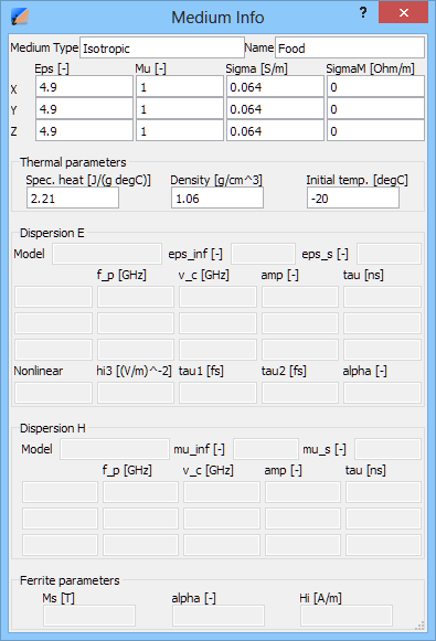
Fig. 2-3 Test Mesh display across food, with Medium Info dialogue for cursor located over food, before the first “heating” run.

While the steady state is being built up, we may open 2D/3D Fields Distribution window (via Fields-2D/3D Fields command or  button in 2D/3D Fields tab) and watch the distribution of electromagnetic and thermal quantities. A set of icons allows selecting the E- and H-field components (three directional as well as total  ), power dissipated per cell , dissipated power density , SAR , enthalpy  and temperature . The    buttons switch between the displays parallel to XY, XZ and YZ planes, while    - between layers. We may amplify  or attenuate  the image, or adjust its amplitude  to fit the window size. We may also switch to Thermal Discrete  display, Thermal Continuous  (in 2D Thermal tab), Art (OpenGL window)    , Points , and Lines (fast)  (all in 2D Surface tab).

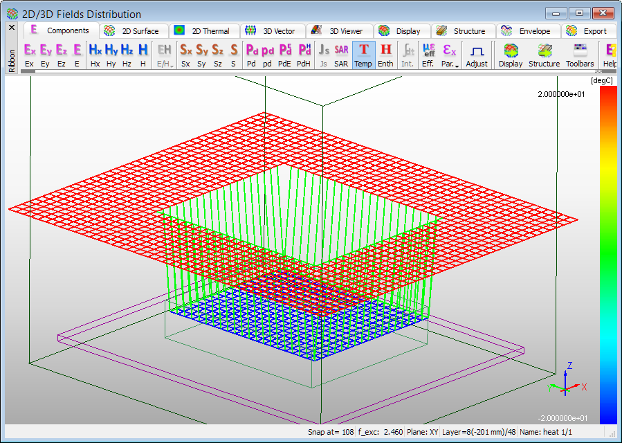
Fig. 2-4 Temperature display across food, before the first “heating” run in 2D Surface Art Lines mode.

The patterns of temperature and enthalpy are trivial at this stage (temperature -20°C in food and +20°C elsewhere, while enthalpy zero all over the scenario). On the other hand, the fields or dissipated power patterns gradually evolve towards the electromagnetic steady state. We deduce that the steady state is reached when:

- dynamically watched fields or power patterns assume repetitive sinusoidally-varying patterns,

- envelopes of these quantities constructed over a few period intervals, starting at various iterations, look identical (see Fig. 2-5),

- values of these envelopes checked at selected locations, e.g. at hot-spots, are equal.

In our case, the steady state is reached after about 4000 iterations. The dissipated power stabilises around the pattern shown in Fig. 2-5, with central hot-spot value of about 0.43 W (red in thermal display as in Fig. 2-6). In Fig. 2-6 load shape has been depicted via Shape button in 2D Thermal tab.

Once in steady state, we may launch the actual Basic Heating Module operation. We invoke Run-BHM-New Heating Pattern command and obtain the BHM Settings dialogue of Fig. 2-7. It allows setting the parameters for the two phases of QW-BHM. During the first phase of Heating pattern construction, the software will be detecting time-average values of dissipated power in each cell. This phase should theoretically last for at least one half of a period, and a longer duration is recommended because of the finite discretisation of time. The QW-Simulator default is 5 periods (see Fig. 2-7). The user may change it and express in either the number of periods or the number of FDTD iterations, which will be mutually re-calculated.

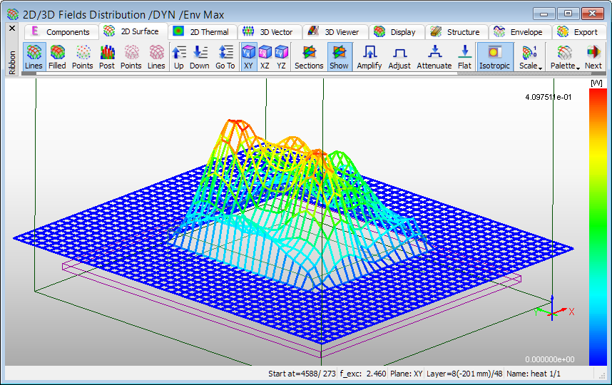
Fig. 2-5 Envelopes of dissipated power across food, constructed for 334 iterations starting at iteration 3674 (upper) and for 273 iterations starting at iteration 4588 (lower).

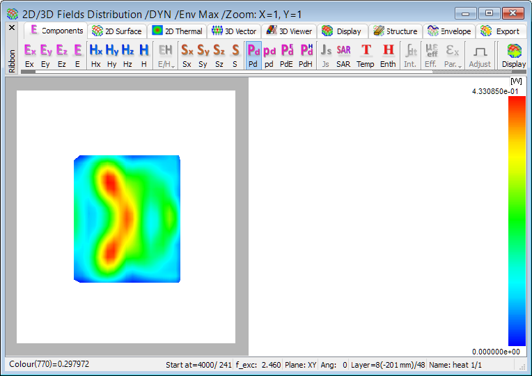
Fig. 2-6 2D Thermal display of dissipated power envelope across food.

During the second phase the above constructed heating pattern will be applied to heat the load for the desired Heating time specified by the user in seconds (Fig. 2-7). QW-BHM performs steps 3, .. 7 explained in Philosophy behind QW-BHM (actually, in default settings of heat.pro, steps 5, 6 are skipped since respective options of heat diffusion and load rotation have not been checked in QW-Editor) and resumes the QW-Simulator (step 8). In 2D/3D Fields Distribution window we may check the updated patterns of enthalpy and temperature, which after this first heating step are naturally proportional to the average heating pattern of Fig. 2-8. Temperature will have increased up to -14°C at some points across the displayed layer of the load. We may also look at the Test Mesh window (), and check that media parameters (using Media Info option) over the food load are different than originally, and varying in space, in accordance with enthalpy variation (permittivity reaching 5.5 and conductivity 0.09 S/m around hot spots).

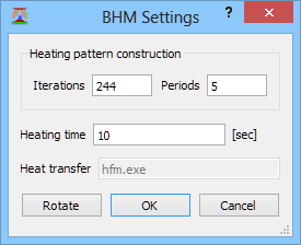
Fig. 2-7 BHM Settings dialogue with default settings.

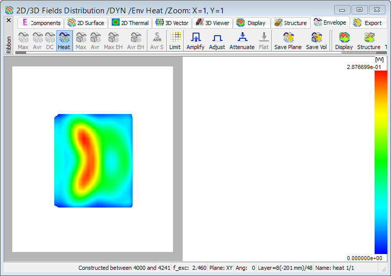
Fig. 2-8 2D Thermal display of dissipated power average envelope across food (constructed between 4000 and 4241 iterations).

Remember that during the phase of heating pattern construction the simulation slows down because at every time-step the software compares the current value of dissipated power in each cell with its time-minimum and time-maximum value for this cell. Except for the case of ideal circular polarisation, these average envelopes will be different from (less than) maximum envelopes of Fig. 2-6. To view the constructed average heating pattern we press  button in Envelope tab (or its keyboard H shortcut) of the 2D/3D Fields Distribution window monitoring dissipated power . Remember that this option is for viewing only, and does not allow any control of the BHM process. It is not available if any quantity other than  is being displayed. In our case the hot-spot value reads about 0.29 W (i.e., indeed less than 0.43 W in Fig. 2-6).

It may happen that the user invokes QW-BHM (via the dialogue of Fig. 2-7) and then wants to interrupt it. In such a case, we call again Run-BHM-New Heating Pattern command (or  button in Run tab) but now (with one BHM process already active) we obtain the BHM Attention dialogue of Fig. 2-9. Pressing No closes this dialogue with no effect on the on-going BHM process. Pressing Yes cancels the current BHM process, resets the calculated heating pattern to zero, and invokes the dialogue of Fig. 2-7 again. We may thus start a new BHM process (setting its parameters and pressing OK) or press Cancel to just continue the EM analysis until the Run-BHM-New Heating Pattern command is called again.

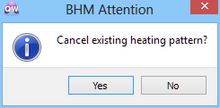
Fig. 2-9 BHM Attention dialogue.

It may also happen that the user first requests a very long time of the heating pattern construction (in the dialogue of Fig. 2-7) and then finds that the pattern has stabilised faster. To interrupt further construction and to move to the actual heating phase, we call Run-BHM-Thermal Effects command (or  button in Run tab). We obtain the BHM Attention dialogue as in Fig 2‑10; pressing Yes moves us through the heating phase (steps 3, 4, 5 of Philosophy behind QW-BHM), pressing No means that the heating pattern construction will continue.

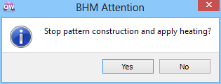
Fig. 2-10 BHM Attention dialogue as obtained via Run-BHM-Thermal Effects command during the on-going heating pattern construction.

Finally, note that the last constructed heating pattern is stored in memory until a new pattern construction is activated. Thus we may apply the last pattern several times. If no BHM process is active, the Run-BHM-Thermal Effects brings up the dialogue of Fig. 2-11, where only the heating time is to be specified. This heating time may be set positive (to add more heating) or negative (to undo media changes). Naturally, if the Run-BHM-Thermal Effects command () is called before any BHM process has been performed, the heating pattern is zero and its application has no effect on the scenario.

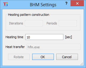
Fig. 2-11 BHM Settings dialogue as obtained via Run-BHM-Thermal Effects command.

It is possible to watch history of temperature and enthalpy at any point within the scenario, versus physical heating time (also called BHM time, and typically of the order of seconds, as opposed to electromagnetic FDTD time, typically of the order of nanoseconds). Invoke 1D Fields window ( button in 1D Fields tab), press Temperature  button or Enthalpy  button in Components tab, and select Time domain  in Domain tab.

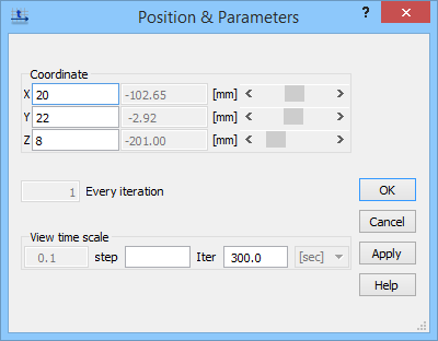
Fig. 2-12 Position & Parameters dialogue for 1D Fields display of time-history of thermal quantities.

This brings up Position & Parameters dialogue of Fig. 2-12. It allows setting the position of monitoring point (expressed in FDTD cells) and the length of View time scale (expressed in seconds). Default time scale resolution is 0.1 sec, as indicated in the dialogue.

A starting point for the time history corresponds to the BHM time at the moment the window is open or its parameters (component, domain, point position, time scale) are modified. If we monitor the results over a time period longer than the View time scale, and the display is dynamic, the displayed sub-period will always be equal to the View time scale, and it will be moving in the window, so that the last sub-period is presented.

The displayed time history of temperature or enthalpy can be saved to a *.de3 file via Save operation () available in Export tab. The header of such a *.de3 file is extended with the following information (with respect to files storing time history of electromagnetic quantities):

! BHM start time [sec] = 2.00000000e+001

! BHM stop time [sec] = 8.00000000e+001

! BHM grid step [sec] = 1.00000001e-001

! BHM save step nb = 7

! BHM save snap at # 8