5.5     Running heat_tune example

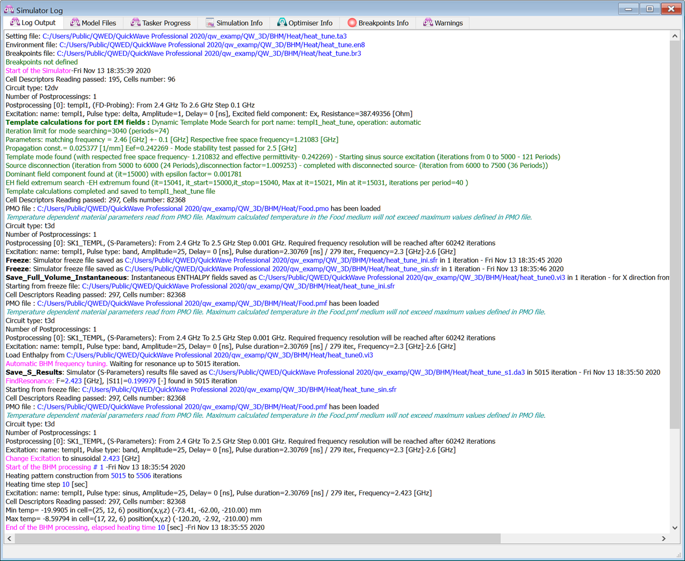
The whole sequence of tasks in heat_tune.ta3 is long (nine BHM iterations). We may monitor its progress and see how many tasks remain to be executed through the Tasker Info tab of Simulator Log, as in Fig. 5.5-1.

Fig. 5.5-1 Tasker Info tab of the Simulator Log window showing progress of heat_tune.ta3 execution.

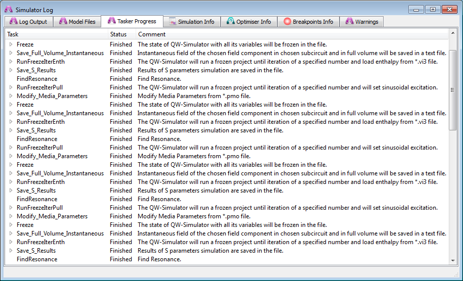
The Log Output tab reports the operations being performed in more detail. Fig. 5.5-2 shows the initial Freeze and Save tasks followed by one full BHM iteration:

- loading the “pulse” scenario (Cell Descriptors Reading...) and updated enthalpy (Load Enthalpy...), and running it,

- saving S-parameter (Simulator results...) and detecting the deepest resonance (Find Resonance...)

- loading the “sinusoidal” scenario (Cell Descriptors Reading...), setting its new excitation frequency (Change Excitation...) and running,

- one basic BHM processing (from Start of the BHM processing to End of the BHM processing),

- freezing the updated scenario with new media parameters, temperature and enthalpy (Simulator freeze...) and saving the new enthalpy (Instantaneous ENTHALPY...).

Fig. 5.5-2 Log Output tab of the Simulator Log window showing details of heat_tune.ta3 execution at its early stage.

Fig. 5.5-3 Temperature and source frequency evolution in heat_tune project, and final temperature pattern across the load (in -20÷0°C scale, in layer 8).

Note that within each BHM processing frame, minimum and maximum temperatures in the scenario are detected and displayed as Min temp=, Max temp=. These are convenient integral quantities for monitoring the whole heating process. After the process is completed, we may trace back the temperature evolution, taking advantage of scrolling the Log Output. This is shown in Fig. 5.5‑3.

What we observe in heat_tune.ta3 is thermal runaway – not a physical effect in this case but a numerically generated one. Note that as a result of source tuning to the resonant frequency (2.243 GHz), the load is heated faster than in the case of heat_auto.ta3 (2.46 GHz) since reflections are reduced from |S₁₁|=0.626 to |S₁₁|=0.1999. Already the first BHM iteration causes maximum temperature of -8.6°, while it was -13.26 for the heat_auto.ta3. The selected heating time step is too long in the phase change region and causes a rapid jump across zero temperature, from -1.14° to 52.29°. The hot spot has much higher conductivity than the lossy area, and hence it then heats up too fast. For physical results, the heating time step should be reduced in this example.