6.3     Rotation example

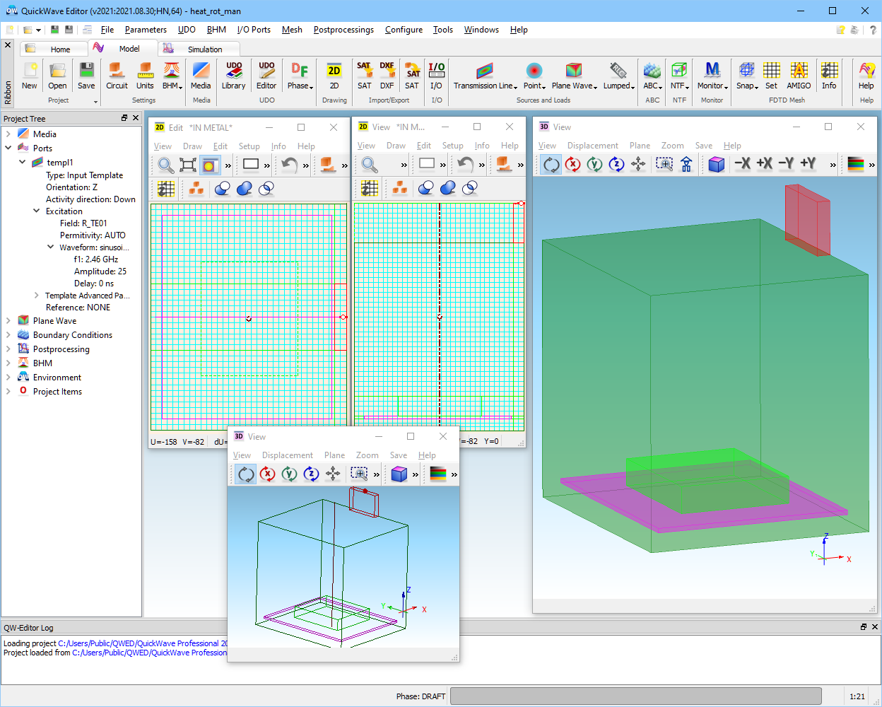
The geometry of the oven has been shown in Fig. 6.3-1.

The goal of the simulation is to obtain the temperature distribution after the sample has been heated for 1 minute with the power of 625 W while the angular speed of the sample around its centre (and the centre of the tray) has been set to 1 rpm (revolutions per minute). The initial temperature of the sample is increased, with respect to heat.pro, to -5°, to facilitate visible heating effects (conductivity at -20° is 0.064 S/m while at -5° it becomes 0.573 S/m ).

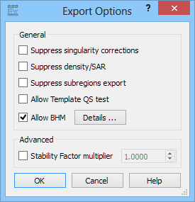
To activate rotation, invoke File-Export Options and in the dialogue make settings as on the left of Fig. 6.3-2. Press  to access the Heating Details dialogue and configure the heating process, as on the right of Fig. 6.3-2. Because the continuous simulation of a rotating load would be a very time- and resources consuming operation, it has been simplified without loosing the computational accuracy by dividing one full revolution of the sample into a number of discrete steps and performing the simulation only for those chosen angles. The number of steps can be selected by the user from the Angular steps drop-down list.

Fig. 6.3-1 The geometry of heat_rot_man.pro example microwave oven containing the load.

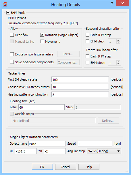
Fig. 6.3-2. The Export Options and Heating Details in heat_rot_man.pro.

For each angle the QW-Editor prepares one *.sh3 file (and a corresponding *.pr3 file) by performing ROTATE (Edit-Reproduce) operation on the object of name specified by the user in the Object name box of the Rotation parameters frame in Heating details dialogue. The rotation is done around an arbitrary point in the xy-plane. The coordinates of the axis of revolution of the sample are defined in the X0 and Y0 boxes.

The information on the number of angular steps together with data about the angular speed of the sample – Speed box – as well as the total heating time – Total heating time box – are used by QW‑Editor to calculate how long the sample should be heated in each of the angular positions and how many thermal iterations are needed:

- Total heating time of 60 sec with Speed of 1 rpm means that one full turn of the Food object will be performed,

- one full turn divided into 12 Angular steps means that will be heated for 5 sec at each angular position,

- this thermal Heating time step = 5 [sec] is displayed in the Heating Details dialogue.

The remaining boxes of the Heating Details dialogue let the user provide Tasker times specified as number of periods of the excitation signal. The frequency of the excitation is displayed in the top frame of the window. As explained in the previous sections of this manual, before the QW-BHM module can be invoked for the first time the electromagnetic steady-state needs to be reached. Only then the simulation of heating can start by performing the first thermal iteration, followed by turning the sample to the next angular position. The number of iterations needed to reach the steady-state has to be provided by the user in the First EM steady state box.

Each of the thermal iterations requires that the data on dissipated power envelope inside the sample be collected. The time needed to collect this information is defined in the Heating pattern construction box. Note that it must be at least half a period, and preferably a few periods, due to finite time resolution.

Consecutive EM steady state box allows specifying how long it is necessary to wait for the next electromagnetic steady state after the previous thermal iteration has been completed. Typically, this is less than the First EM steady state by a factor of ten.

After all the boxes in the Heating Details dialogue have been filled with the necessary parameters of the simulation, the user should press  button. This will close the dialogue window. Now, in order to start the simulation it is enough to press the Export, Run & Start  button on the QW-Editor tool bar. The QW-Editor will prepare the *.sh3 and *.pr3 files as well as the tasker heat_rot_man.ta3 file instructing QW-Simulator about the tasks to be performed.

QW-Simulator starts performing its tasks while we may inspect the contents of heat_rot_man.ta3 file via View-Edit Ta3 File. The beginning of the tasker file obtained for the example circuit based on the parameters shown in Fig. 6.3-2 is presented in Fig. 6.3-3. It covers the initial template generation and the first two thermal iterations.

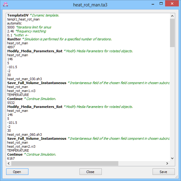
Fig. 6.3-3 Fragment of the tasker file heat_rot_man.ta3 (two thermal iterations) prepared byQW-Editor based on the parameters from Heating Details dialogue and displayed in QW-Simulator.

RunIter command with 4897 iterations parameter brings the analysis to the first estimated steady state (period=1/f=0.4ns, dt=0.0083 as accessed in Simulation Info, 48.97 iterations/period*100 periods=4897 iterations).

“Thermal” tasks are contained in the command Modify_ Media_Parameters_Rot. It is very similar to the command Modify_Media_Parameters already described. The command Modify_Media_Parameters_Rot first activates constructing the heating pattern (for 3 periods * 48.97 iterations/period=146 iterations). Then it applies this heating pattern to heat the load for 5 sec, and updates enthalpy, temperature and media parameters. Finally, it rotates the resulting enthalpy and temperature distributions by angle 30° around point (-101.5, -2) in the xy plane. At the same time, the new geometry is read by the QW-Simulator from heat_rot_man_030.sh3 file.

The only difference between the syntax of Modify_Media_Parameters_Rot and Modify_Media_Parameters commands are new parameters added – the coordinates of the axis of revolution of the sample, the angular step, and the name of the *.sh3 file containing the geometry at the new angle.

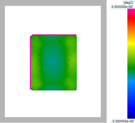
Fig. 6.3-4 Temperature in heat_rot_man project, and final temperature pattern across the load (in -5÷0°C scale, in layer 8).

The tasker file generated automatically by the QW-Editor also contains commands instructing the QW-Simulator to save distribution of the temperature field after each thermal iteration, over the full volume of the project. This feature helps the user keep track of the evolution of the temperature field during heating. However, if the heated sample occupies just a small part of the volume, the saved files contain a lot of redundant information. In such a case, the user may replace Save_Full_Volume_Instantaneous command with Save_Volume_Instantaneous over a specific sub-volume.

After reaching the first steady state at iteration 4897, and performing the additional 146 iterations to build the heating pattern, QW-Simulator is at iteration 5043. Now it needs to run for 10 more periods, i.e., 489 iterations. Therefore the parameter of the Continue command is 5532=5043+489. This will be the second EM steady state, whereat the second Modify_Media_Parameters_Rot command will be performed.

This sequence of Modify_Media_Parameters_Rot, Save_Volume_Instantaneous, Continue is performed 12 times, for the 12 angular positions. Note that the last Continue command has parameter 0, which means that EM simulation will continue until stopped by the user. On the disk, the 12 *.vi3 files will be available for the inspection of temperature evolution. After exiting QW-Simulator, information from the Simulator Log will be saved in heat_rot_man_log.htm (if so chosen in Configure-Preferences dialogue), which allows tracking the evolution of minimum and maximum temperature in the scenario.