5.3     Sensitivity to the tuning

Before using the BHM regime with automatic frequency tuning to the deepest resonance, we should check whether a particular scenario, with the particular media characteristics, may significantly “pull” the resonance.

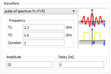
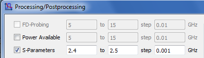
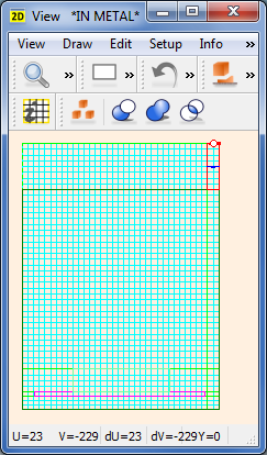
Fig. 5.3-1 2D view of heat_pulse.pro together with relevant parts of Select Element, Edit Transmission Line Port and Processing/Postprocessing dialogues.

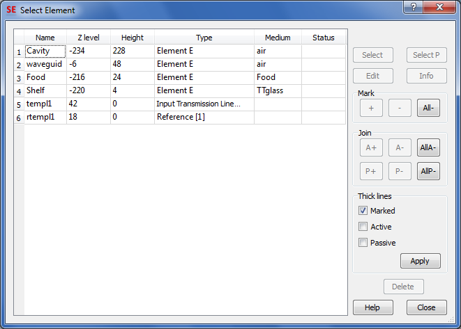
Consider ..BHM\Heat\heat_pulse.pro example. It is essentially equivalent to heat.pro, except that the source has been changed to the one taking part in S-parameter extraction. As show in Fig. 5.3-1, the source templ1 now has its reference plane rtempl1. Pulsed excitation between 2.3 GHz and 2.6 GHz is applied, and S-parameters are extracted between 2.4 GHz and 2.5 GHz.

Note that the source tuning will be performed within the post-processing band, i.e., between 2.4 GHz and 2.5 GHz and this band has been selected as reflecting typical magnetron spectrum variations within a 50 MHz margin. The band of excitation cannot be narrower and is usually set equal to the post-processing one. Here it is set somewhat wider for fast manipulating with the post-processing band and for somewhat faster launching of the pulse (knowing that no high-Q resonances are excited within the source but outside the post-processing band).

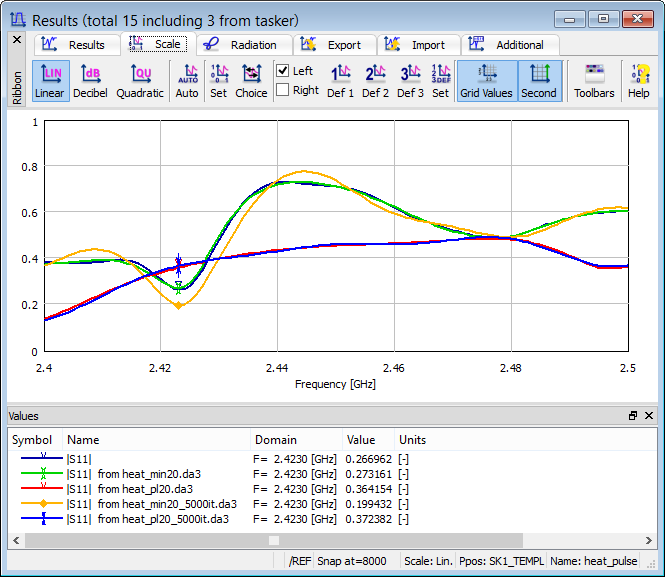
Fig. 5.3-2 Return loss characteristic of heat_pulse.pro: green – steady state with default parameters (food at -20 deg), red – steady state but with food medium at +20 deg, navy – after 8000 iterations with default parameters, yellow – after 5000 iterations with default parameters, blue – after 5000 iterations with food medium at +20 deg.

In Fig. 5.3-2 we check two aspects:

- Whether thermal variation of media parameters in this scenario may change the resonant frequency is any observable way. The answer is yes, as shown by the green and red curves. For the food medium at the initial temperatures of -20 deg we obtain the green curve, with the best matching of |S₁₁|=0.273 at 2.423 GHz. When the whole food load heats up to +20 deg (and all other scenario parameters remain unchanged), the matching improves due to higher food losses (see food.pmo file), the resonance is less pronounced and shifted below 2.4 GHz.

- Whether the first steady state is indeed reached after approximately 5000 FDTD iterations, which was assumed in creating the tasker files of Batch operation. In the presence of resonances, frequency-domain S-parameters in pulsed FDTD regime may converge slower than time-domain envelopes of field and power in sinusoidal FDTD regime. The green and red curves described above have been obtained for reference after a long simulation time (15000 FDTD iterations amounting to about 300 periods at the centre frequency). The pulsed simulation with a lossy load – food at +20 deg – is shown to converge to the steady state even faster than the 100 periods assumed in Batch operation (see blue curve overlapping with the red one). The pulsed simulation with the smallest losses for this scenario - food at -20 deg – shows minor oscillations after the 100 periods (yellow curve) and practically stabilises after 160 periods (navy curve). However, since the yellow curve correctly depicts the resonant frequency, and differs in the matching level only, the First EM steady state setting of 102 periods will be maintained for the BHM regime with source tuning.