
2.6.4 Illumination with Gaussian beams
Illumination with a plane wave well approximates these physical cases where a spot size of the illuminating wave is larger than the scattering object’s dimensions. There are, however, numerous cases where the actual finite size of the spot must be considered and may be smaller than the object’s dimensions. This happens in measurements and scatterometry techniques.
Solutions to the Maxwell equations in free space that provide finite spots are Gaussian beams. The so-called 3D Gaussian beam propagating along a particular dimension focuses in the other two dimensions around a point called a neck centre, creating a Gaussian-shaped spot of size called a neck diameter; it then de-focuses beyond the neck. The so-called 2D Gaussian beam propagates along one dimension, focuses in the second dimension, and remains invariant along the third.
Both types of Gaussian beams are supported in QW-3D. They are generated at the same boxes as previously the plane wave (plane wave box). The choice of the illuminating wave is made at the Add Plane Wave/Edit Plane Wave dialogue level. Fig. 2.6.4-1shows Edit Plane Wave dialogue for free space illumination:
- TEM, B3D and B2D radio buttons allow choosing between plane wave, 3D Gaussian beam and 2D Gaussian beam, respectively.
- Phi, Theta and Polarisation angles have the same meaning for all waves. Thus the setting shown in Fig. 2.6.4-1correspond to the wave propagating along +Z axis with Ex, Hy fields (being the only fields in a plane wave, and the dominant ones in Gaussian beams).
- NeckX, NeckY, NeckZ are coordinates of the neck centre and N_dia is neck diameter.
- For the 2D Gaussian beam one more parameter is defined under Beam 2D. Angle of variation determines the direction in which Gaussian shape is produced. It is defined analogously as polarisation (see Plane wave without the scatterer) and its versor is given by:
[cosAngcosPhicosTheta - sinAngsinPhi, cosAngsinPhi cosTheta + sinAngcosPhi, - cosAng sinTheta]
Fig. 2.6.4-1 The Edit Plane Wave dialogue in the plg.pro example.
The plg.pro example demonstrates a 3D Gaussian beam propagating along the z-axis, with the dominant Ex field. Fig. 2.6.4-2shows instantaneous E-field along the direction of propagation (left) and around the neck (right). Focusing at the neck is clearly visible. Fig. 2.6.4-3shows the field envelope. It reveals that the neck is actually shifted by some 10 mm down from the requested position. This results from an approximation made in exciting the wave, namely, neglecting changes of the electric field angle in space. This approximation works well for neck diameters of several wavelengths or more, while in the present example it equals only one wavelength.
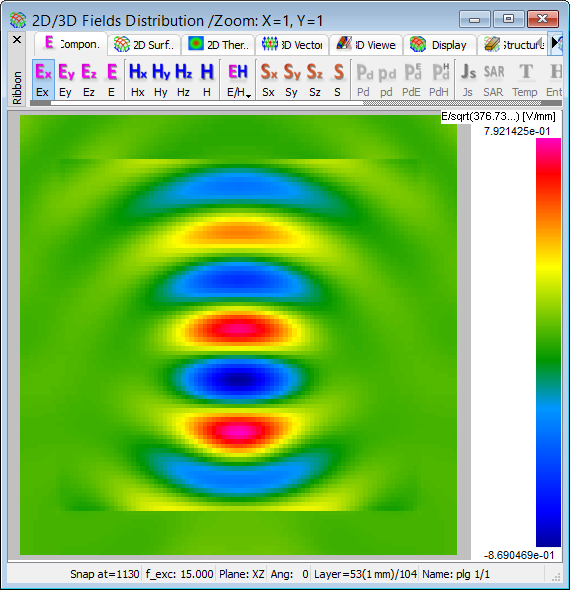
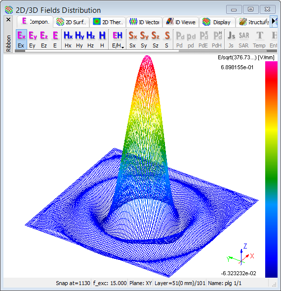
Fig. 2.6.4-2 Instantaneous Ex-field in the plg.pro example: in the central vertical plane and around the neck.
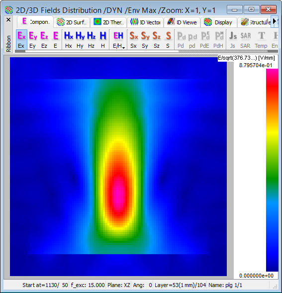
Fig.UG 2.6.4-3 Ex-field envelope in the plg.pro example, in the central vertical plane.