
2.6.1 Plane wave without the scatterer
We shall now consider a simple example, which consists of:
· cubic volume of free space (cube side = 40 mm), with absorbing exterior boundaries,
· a surface for near-to-far transformation (NTF box) with each wall placed 4 mm from an absorbing boundary,
· a surface for plane wave excitation (plane wave box) with each wall placed 10 mm from an absorbing boundary.
In such a structure we shall observe plane wave propagation at 10 GHz. A view of this project (named ..\Scattering\Plwave\plw1.pro) in QW-Editor, in 2D Window in the XY-plane and 3D Window is shown in Fig. 2.6.1‑1.
The project is ready to be used. However, for tutorial purposes we shall explain all the steps needed to prepare such a project from scratch, save it as plw1b.pro, and run it.
Fig. 2.6.1-1 QW-Editor display of plw1.pro.
STEP 1: setting up a new project
On the entry to QW-Editor you will see the last project developed by previous users of the software. Please select: New to move to your new project. The default name noname will appear in the title bar. Now select Save as (in Hometab), and write the name of your project into a dialogue box; let the name be: plw1b.pro.
Note that the windows of the previous project have remained open. Close the windows you do not need. In fact, you will need at least one 2D Window for drawing, and a few additional 2D and 3D Windows may be helpful for visualisation. Please open one 2D Window and one 3D Window clicking successively over each of these two buttons: ![]()
![]() , in Hometab.
, in Hometab.
At this stage you should decide what units will be used. To set the units, invoke Units (![]() button in Modeltab) and select an appropriate radio button in the dialogue. In this project we select mm (millimetres).
button in Modeltab) and select an appropriate radio button in the dialogue. In this project we select mm (millimetres).
STEP 2: defining the type of the structure
Open Circuit dialogue. Please make sure that the settings in the appearing dialogue are as presented in Fig. 2.6.1-2and click OK. It is important to select here the circuit type: 3D and default medium: air. Description is not obligatory but we recommend as a good habit to include a meaningful description of the project. The other fields are irrelevant in this particular project.
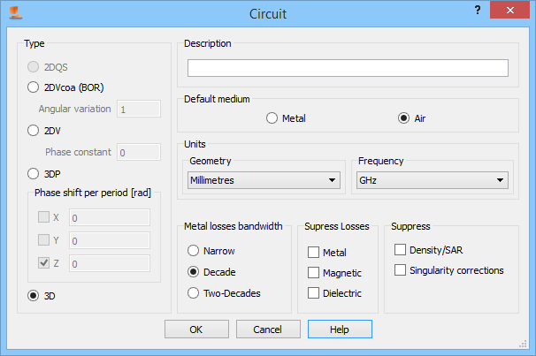
Fig. 2.6.1-2 Circuit dialogue settings for plw1.pro.
Notethat since the default medium is air, expression *IN AIR* appears in the 2D Window. Also a background colour of the 2D Window is that defined in 2D View Options dialogue.
STEP 3: drawing the structure
We press the ![]() button in 2D Window and select plwntf.udo from the object library: boxes. A UDO header appears, in which we are supposed to make the settings as presented in Fig. 2.6.1-3 (left). Then we press Draw.
button in 2D Window and select plwntf.udo from the object library: boxes. A UDO header appears, in which we are supposed to make the settings as presented in Fig. 2.6.1-3 (left). Then we press Draw.

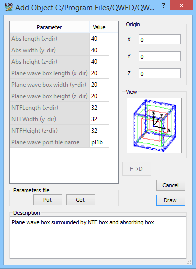
Fig. 2.6.1-3 Header of plwntf.udo: during preparation of the project and before the pl1b.iop file is prepared (left) and with parameters eventually used in plw1.pro and plw1b.pro.
Our new project plw1b.pro now includes all the elements available in plw1.pro. We can press the ![]() button (in 2D Window) to see the list of elements as presented in Fig. 2.6.1-4. It shows that the absorbing box is a cube with opposite vertices at (0,0,0) and (40,40,40), the NTF box is shifted by 4 mm from each absorbing wall and the plane wave box with is a cube of the size 20 mm situated inside.
button (in 2D Window) to see the list of elements as presented in Fig. 2.6.1-4. It shows that the absorbing box is a cube with opposite vertices at (0,0,0) and (40,40,40), the NTF box is shifted by 4 mm from each absorbing wall and the plane wave box with is a cube of the size 20 mm situated inside.
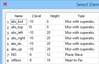
Fig. 2.6.1-4 List of elements of plw1.pro and plw1b.pro.
STEP 4: setting up the mesh
The circuit is meshed with default cell size equal 1 mm. We will maintain this default mesh.
STEP 5: defining simulation parameters
Note that when setting the UDO parameters of Fig. 2.6.1-3(left) we have made a special choice of plane wave port file name. We have chosen it to be NO. According to the description of the plwntf.udo, such a choice means that the software will not be looking for a specific file with port parameters. We have not prepared such a file yet and thus an attempt to read it would result in a UDO interpreter error. The declaration of ”NO” allows us to prepare such a file in a convenient way to be able to use it at further calls to plwntf.udo.
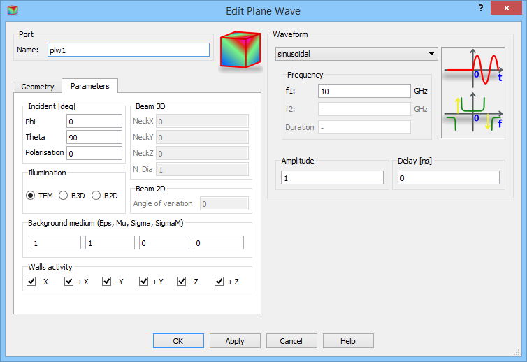
Fig. 2.6.1-5 Edit Plane Wave dialogue with parameters for the considered plane wave example.
Invoke Edit Plane Wave. Set the parameters as displayed in Fig. 2.6.1-5. Now press Put and store the port parameters in the project directory under a chosen name, for example pl1b.iop (*.iop extension is added automatically).
Press ![]() button (in 2D Window) and double-click ntfplw on the list of objects. The header as in the left part of Fig. 2.6.1-3 comes up. Modify Plane wave port file name as shown in the right part of Fig. 2.6.1-3 and press OK. Upon each consecutive modification of the UDO the software will read the pl1b.iop file and maintain excitation parameters as in this file.
button (in 2D Window) and double-click ntfplw on the list of objects. The header as in the left part of Fig. 2.6.1-3 comes up. Modify Plane wave port file name as shown in the right part of Fig. 2.6.1-3 and press OK. Upon each consecutive modification of the UDO the software will read the pl1b.iop file and maintain excitation parameters as in this file.
Note that we have three angles to be chosen:
- j (Phi) – azimuthal angle of the direction of wave propagation
- q (Theta) – elevation angle of the direction of wave propagation
- Polarisation – polarisation angle of the electric field.
With all these angles set to zero, the incident wave travels along the z-axis and its electric field vector is oriented along the x-axis. In general, the direction of propagation determines a modified z’ axis, and the electric field orientation determines a modified x’ axis, of the modified x’y’z’ coordinate system obtained from the original xyz coordinate system by rotation with Euler angles Phi, Theta, Polarisation in the ZYZ Euler convention. For more details about Euler angles please refer to the final part of Two dipoles in free space excited in phaseand the figure therein.
An alternative explanation of the three angles is as follows. The direction of wave propagation is inclined by angle Theta from z-axis towards x-axis, and rotated by angle Phi from x-axis towards y-axis. Consider this direction to be ir direction of a spherical coordinate system, at the point where the wavefront first reaches the sphere. With Polarisation equal zero, the electric field will be oriented along iqdirection at this point. Otherwise Polarisation is the angle between the unit vector iqand the electric field vector measured in the plane of unit vectors iqand ij.
Mathematically, the versor in the direction of wave propagation is:
[cosPhi sinTheta, sinPhi sinTheta, cosTheta]
and the versor in the direction of the electric field vector is:
[cosPol cosPhi cosTheta - sinPol sinPhi, cosPol sinPhi cosTheta + sinPol cosPhi, - cosPol sinTheta]
With the settings of Phi=0, Theta=90 and Polarisation=0 in Fig. 2.6.1-5the wave propagates in the +x direction and positive E-field is in the –z direction.
STEP 6: exporting project data
First click ![]() to save the project. It is recommended to run firstly plw1.pro example and then the newly prepared project to compare the results. Click
to save the project. It is recommended to run firstly plw1.pro example and then the newly prepared project to compare the results. Click ![]() to export the files, call QW‑Simulator, and start the simulation.
to export the files, call QW‑Simulator, and start the simulation.
STEP 7: running FDTD simulation
After a few hundred of iterations press ![]() button in 2D/3D Fields tab of QW-Simulator to invoke 2D/3D Fields Distribution window. The display as in Fig. 2.6.1-6appears. Note that plane wave is incident in X (Phi=0 deg and Theta=90 deg) direction. Stop the simulation by clicking
button in 2D/3D Fields tab of QW-Simulator to invoke 2D/3D Fields Distribution window. The display as in Fig. 2.6.1-6appears. Note that plane wave is incident in X (Phi=0 deg and Theta=90 deg) direction. Stop the simulation by clicking ![]() button in Runtab of QW-Simulator and return to QW-Editor.
button in Runtab of QW-Simulator and return to QW-Editor.
Now return to STEP 5, introduce Phi=45 and press OK (those seetings are made in plw1m1.pro example). Then click ![]() button to run the simulation for new excitation. After a few hundred of iterations press
button to run the simulation for new excitation. After a few hundred of iterations press ![]() button. The image of Fig. 2.6.1-7appears. Now it is visible that the plane wave is incident in Phi=45 deg and Theta=90 deg direction.
button. The image of Fig. 2.6.1-7appears. Now it is visible that the plane wave is incident in Phi=45 deg and Theta=90 deg direction.
If you run newly prepared project, after a few hundred of iterations press ![]() button in 2D/3D Fields tab of QW-Simulator to invoke 2D/3D Fields Distribution window. Press
button in 2D/3D Fields tab of QW-Simulator to invoke 2D/3D Fields Distribution window. Press ![]() button in 2D Surface tab until Layer: 20/41 appears in the window status bar, and press
button in 2D Surface tab until Layer: 20/41 appears in the window status bar, and press ![]() button in Componentstab to see the picture as in Fig. 2.6.1-6.
button in Componentstab to see the picture as in Fig. 2.6.1-6.
Stop the simulation by clicking ![]() button in Runtab of QW-Simulator and return to QW-Editor.
button in Runtab of QW-Simulator and return to QW-Editor.
Now return to STEP 5, introduce Phi=45 and press OK. Then click ![]() . After a few hundred of iterations press
. After a few hundred of iterations press ![]() button. The image of Fig. 2.6.1-7appears.
button. The image of Fig. 2.6.1-7appears.
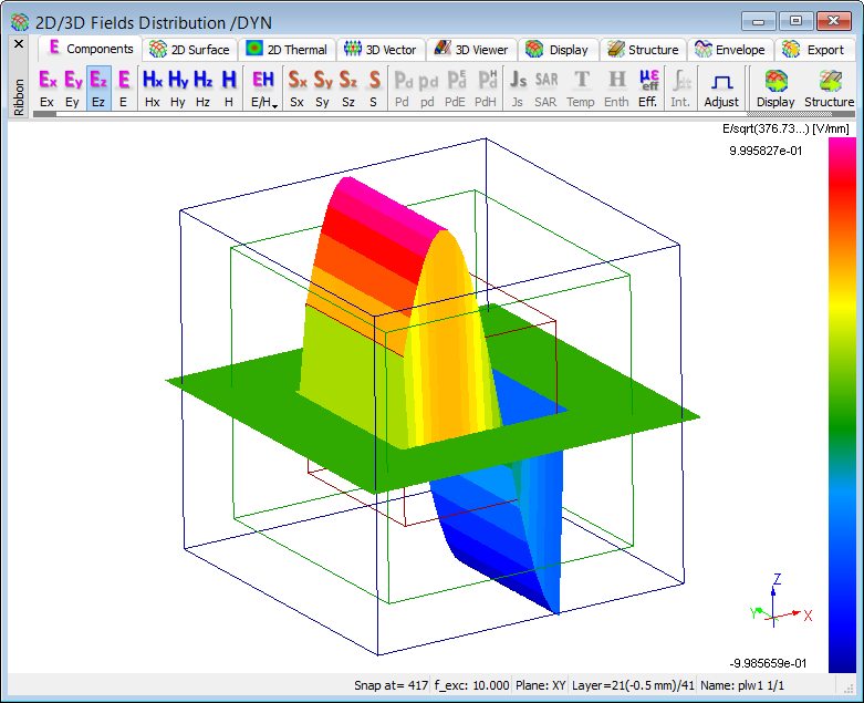
Fig. 2.6.1-6 Ez component of plane wave excitation in the first experiment with plw1.pro.
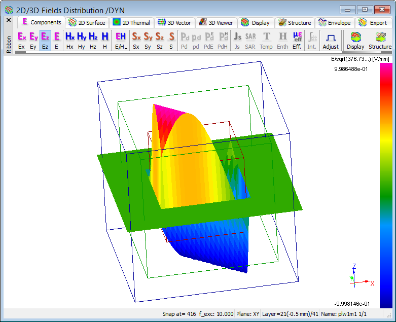
Fig. 2.6.1-7 Ez component of plane wave excitation in the second experiment with plw1m1.pro.