3.2.1.         UDO creation

In the UDO script format we can distinct four main blocks:

-        Comment block – here a short description of the structure, which UDO script defines, is given

-        Header – where parameters definition is made,

-        Test block – where the security formulas can be defined,

-        Body – where the geometry, ports, media, etc. can be defined.

We will now, step by step, get through UDO script preparation, based on ant3 project and its ant3.udo base script. We open UDO Editor and create new file called ant3.udo. Next, the following steps needs to be accomplished:

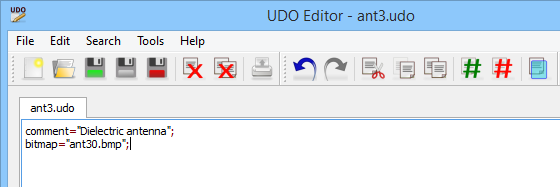
1.     Firstly we define the comment block. For that purpose we use comment command and then we put in quote a short description of the structure that this UDO script describes (Fig. 3.2-4). This description will appear in the Add Object window of QW-Editor (Fig. 3.2-5), as marked with red, which is used whenever we want to draw/redraw the udo (through Draw->UDO Library and Edit‑>Select Object options of 2D window of QW-Editor).

Using the bitmap command we can indicate the *.bmp file with the graphic that will appear in the View field of Add Object window (blue in Fig. 3.2-5) and in the window listing the available UDO scripts after invoking Draw->UDO Library option (Fig. 3.2-6) of QW-Editor.

Fig. 3.2-4. Comment block for the ant3.udo.

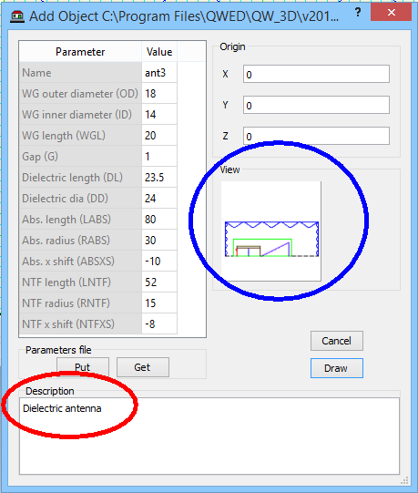
Fig. 3.2-5. Add Object window.

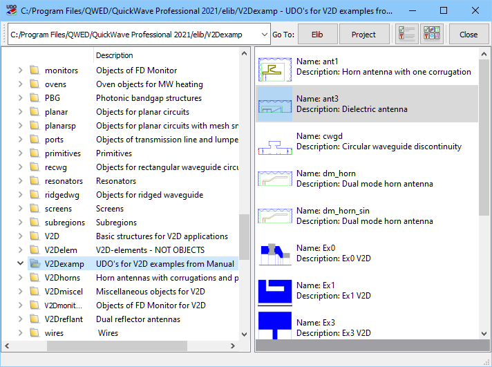
Fig. 3.2-6. A window appearing after invoking Draw->UDO Library option in QW-Editor.

2.     In the next step we need to create the header. Here, all the variables (dimensions of the structure, material parameters, etc.) that we suspect we would like to change during the design process should be defined as UDO script parameters using PAR command:

PAR (<description>,< name>,<default value>);

where:

<description> - parameter description. If the description contains operator chars, the text has to be delimited with apostrophes.

<name> - case sensitive name of parameter which can be used in expressions within the udo script body.

<default value> - initial value for parameter, it can be a number or string.

Attention: Note that the description of all UDO commands is given in Syntax of the User Defined Object (UDO) language chapter of QW-Editor manual.

In the case of ant3 antenna all the geometrical parameters (as given in Fig.3.2-2 and Table 1) will be defined using PAR command. The declaration of those parameters is shown in Fig.3.2- 7.  As a first parameter we define the main object name (main object is considered to contain the body of the UDO script), which is “ant3”.  Each of the geometrical parameters has its description, name given according to definition in Fig.3.2-2, and the default value is assigned according to Table 1.

At the moment we do not have other variables to be declared as PARameters, thus we can close the header block with ENDHEADER command.

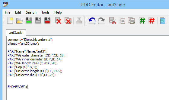
Fig. 3.2-7. Header of the UDO script with parameters defined.

3.     Next step is determining the Test block conditions. In the Test block we can define conditions that, if not fulfilled, will stop (with the information displayed in QW Project Info and QW-Editor Log windows of QW-Editor) the drawing/redrawing UDO operation invoked from QW-Editor.

In general, here we may for example put conditions that prohibit setting negative values for structure dimensions, etc.

In this particular case we will make the condition that prevents drawing the structure in situation where the outer waveguide dimeter (OD) is smaller than inner waveguide diameter (ID). Those conditions are defined using TEST command:

TEST (<logical expression>,<message text>);

where:

<logical expression> - expression which should be true,

<message text> - text displayed if logical expression is false.

The test expression is defined as shown in Fig. 3.2-8. When drawing/redrawing the UDO script, QW-Editor will check if OD parameter is bigger than ID; if yes it will continue with performing operations declared with further UDO commands; if the condition is not obeyed the warning “OD>ID!” will appear in the QW-Editor in QW Project Info and QW-Editor Log windows.

Note that the TEST commands can but do not have to be determined in the UDO script.

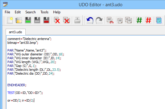
Fig. 3.2-8. UDO script with Test block added.

Directly under the header and test blocks, the mathematical operation may be declared (those operations may be also declared inside the Body block).

Here we declare two simple equations as given in Fig. 3.2-8. In header block we have defined outer and inner diameter of the waveguide. Since we will be drawing only half of a long section of the antenna it will be convenient to define the outer and inner radius of the waveguide as new variables (or and ir) and use them further when defining the structure’s geometry.

Now we can proceed with defining the UDO script body.

4.     Body of the UDO script contains all geometry elements, simulation objects, etc.

It starts with OPENOBJECT command and is treated as main object. The OPENOBJECT command requires object name parameter given as a string in quote or as a UDO parameter like in this case. The Body block (main object) should be ended with CLOSEOBJ command, which will be put at the end of the Body definition.

Now we can proceed with antenna’s elements definition using ELEMENT, NEWLINE, ADDY, and ADDX commands. We will start with the cylindrical waveguide. According to Fig. 3.2-3 (showing the half of antenna’s long section) and the rule saying that we need to draw the element by giving the coordinates of the following points, the waveguide shall be drawn as a rectangle, defined by four points with coordinates as given in Fig. 3.2-9 (defined with respect to (0,0) point).

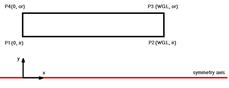
Fig. 3.2-9. Half of a cylindrical waveguide long section with point coordinates indicated.

For the purpose of drawing the geometrical element we use ELEMENT and ENDELEM commands:

ELEMENT (<level>,<height>,<type>,<medium name>,<name>,<spin/wire>) - Start of element frame, where:

<level> - level of element base, usually relative to predefined origin variable z,

<height> - height of element, for combined elements is forced to zero,

<type> - type of element:

0 - simple element,

5 - bottom of combined element,

6 - cover of combined element.

<medium name> - name of element medium (if there is no such medium air is forced),

<name> - name of element,

<spin/wire> - orientation of element edge or wire marker:

IN, INe, INn, INs - medium fills inside the defined left (counter-clockwise) oriented contour. These are typical settings practically for all applications except of wires. IN and INe enforce E-plane of the FDTD grid at the level of the bottom and top of the element. INn enforces neutral plane (either E-plane or H-plane) of the FDTD grid at the level of the bottom and top of the element. INs results in a suspended element, which does not force any mesh snapping planes; instead it is approximated with suspended mesh snapping planes. Additionally, lowercase letter d, l or h can be appended to IN (and INe, INn, INs) options to define classes of AMIGO priorities (respectively disabled, hard edges (lines), hard).

OUT - medium fills outside the defined left (counter-clockwise) oriented contour. Note that this option is not recommended for a general use.

WIRE - element is a wire line. The programmer has to ensure a proper shape of such an element. The line describing the wire shape does not need to be closed. Inside the frame of the element declared as WIRE, there may be a declaration of its diameter as presented below.

ENDELEM - End of element frame.

As it was noted in part 1 of this chapter, in case of QW-V2D all elements should be defined at Z level=0 and height=1, thus first two parameters in the ELEMENT command are z (z+0=z) and 1 (Fig. 3.2-10). Next, the element type should be determined. Note that in QW-V2D only simple element type is used, thus the next parameter is set to 0. The waveguide should be made of metal thus the following parameter will be metal. Note that in QuickWave there are three media that are by default available and do not have to be additionally defined in the UDO script (or directly in the QW-Editor). Those are: metal (PEC), air, and open (PMC). The names of those media are unique and are used for the medium declaration. Other media, if necessary for assigning to the element/object, need to be defined by the user (it will be further explained). We will name the element with waveguide and assign the spin to be IN.

We can now draw the waveguide, point by point. Every drawing must start with NEWLINE command:

NEWLINE (<x1>,<y1>,<x2>,<y2>) - Insert line from point (x1, y1) to point (x2, y2).

Thus we have NEWLINE(x, y+ir, x+WGL, ir);

The following sections may be drawn using ADDLINE command:

ADDLINE (<x3>,<y3>) - Insert line from previous point to point (x3, y3).

Or

ADDX and ADDY commands:

ADDX (<dx>) - Insert a line parallel to X-axis from (x2,y2) to (x2+dx, y2).

ADDY (<dy>) - Insert a line parallel to Y-axis from (x2,y2) to (x2, y2+dy).

We will use the second option where dy= or-ir and dx=0-WGL=-WGL: ADDY(or-ir); and ADDX(-WGL);

The last section (between P4 and P1) is drawn using CLOSELINE command:

CLOSELINE - Insert line from previous point to (x1, y1) point of the last NEWLINE.

At the end we put ENDELEM command and in such way we have drawn the waveguide element.

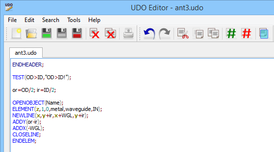
Fig. 3.2-10. Body of the UDO script – waveguide element.

In the next step we will draw the dielectric cylinder filling the waveguide. A backup sketch for this element is shown in Fig 3.2-11. This element also has a shape of simple rectangle (when rotated around symmetry axis it will be a cylinder).

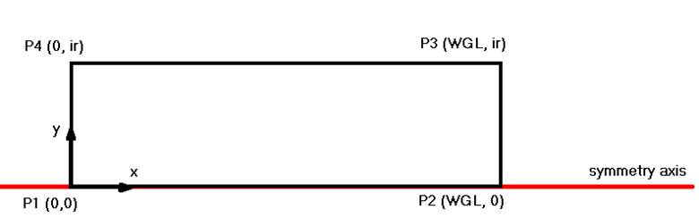
Fig. 3.2-11. Half of a long section of dielectric filling the waveguide, with points coordinates indicated.

We need to remember in this case that this element is made of dielectric material and we need to declare this material and define its parameters. For that purpose the INSERTMEDIUM and MEDIUMPAR commands are used:

INSERTMEDIUM (<mediumname>, <type>) - Inserts a new medium into the project, if medium of the same name does not exist.

The parameter type options are: ISOTROPIC, ANISOTROPIC, DIELECTRIC_DISPERSIVE, DIELECTRIC_DISPERSIVE_ANISOTROPIC, META_MATERIAL, FERRITE, METAL, PEC, PMC.

MEDIUMPAR (<mediumname>, <epsx>, <mux>, <sigx>, <msigx>, <epsy>, <muy>, <sigy>, <msigy>, <epsz>, <muz>, <sigz>, <msigz>, <density>) - Change the parameters of the medium "mediumname" to those specified by the subsequent parameters. These parameters should be self-explaining by comparison with those displayed in the Parameters-Media dialogue window. Note that the above instruction will not change the type of the medium. Thus for example if the considered medium was declared in the Parameters-Media dialogue (or in INSERTMEDIUM command) as isotropic, the values of epsy, epsz, muy, muz etc. declared as arguments of MEDIUMPAR will be ignored. This command allows using material permittivity, permeability, etc. as UDO parameters. Thus it allows for example changing medium parameters in a quasi-continuous way, as variables modified in a loop.

Fig. 3.2-12 shows the definition of the dielectric cylinder filling the waveguide (green frame). Thus we declare the dielectric medium as isotropic dielectric (ISOTROPIC) and name it “diel3_6” using the INSERTMEDIUM command, and define its parameters with MEDIUMPAR command according to data given below Table 1.  The geometry of the dielectric cylinder filling the waveguide is drawn in the similar way as it was in case of waveguide (Fig. 3.2-12).

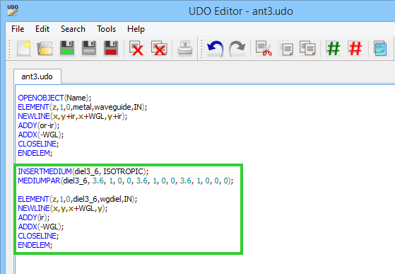
Fig. 3.2-12. Definition of dielectric element filling the waveguide.

Next step is to draw the dielectric cone. Half of a cone’s long section has a shape of triangle. The sketch showing the points’ coordinates is shown in Fig. 3.2-13.  The procedure of drawing the dielectric cone is exactly the same as in case of dielectric cylinder filling the waveguide: firstly the medium and its parameters need to be determined and then the geometry of the cone is defined. The commands describing the dielectric cone are shown in Fig. 3.2-14 (red frame).

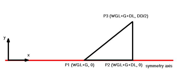
Fig. 3.2-13. Half of a long section of dielectric cone with points coordinates indicated.

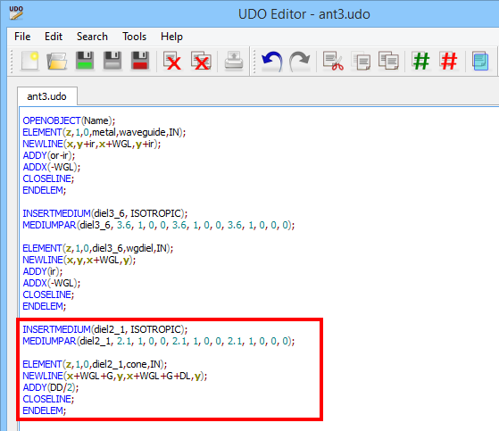
Fig. 3.2-14. Definition of the dielectric cone.

The antenna has been already defined, now we need to introduce two additional elements: excitation port and NTF box (with absorbing box and magnetic symmetry plane).

Firstly we will introduce the excitation port. For that purpose we will take advantage of the UDO library and use a ready-to-use port object (port2dv) available there. In QW-Editor (in 2D window) we choose Draw->UDO Library option and we get window as in Fig. 3.2-15. We press Elib button and the window shows the UDO library directory with several folders (on the left) where ready-to-use UDO scripts are grouped. We choose V2D folder by clicking on it and available UDO objects appear on the right. The one of our interest is port2dv. In general, the objects from UDO library (and any other UDO objects defined in external UDO scripts) can be used in our UDO script using CALL command:

CALL(<path>,<par1>,<par2>,..,<parn>,<parx>,<pary>,<parz>,<N>);

<path> - path to *.udo file for nested object (the path is indicated with respect to the root directory of elib)

<par1>..<parn> - n parameters of nested object, in the place of each parameter we can put a value, a variable or an arithmetic expression,

<parx>,<pary>,<parz> - origin of nested object,

<N> - number of parameters of this CALL excluding <N> (N=n+4)

The list of parameters is unique for every UDO script, thus the CALL command will be different.

For every UDO object, UDO library delivers a hint concerning the CALL command syntax. This hint can be found in the Description available under right mouse button menu (Fig. 3.2-16). When the user chooses Description, the description as in Fig. 3.2-17 will be opened in the web browser. It contains the description of all parameters that need to be determined for this object and the syntax of appropriate CALL command (red arrow).

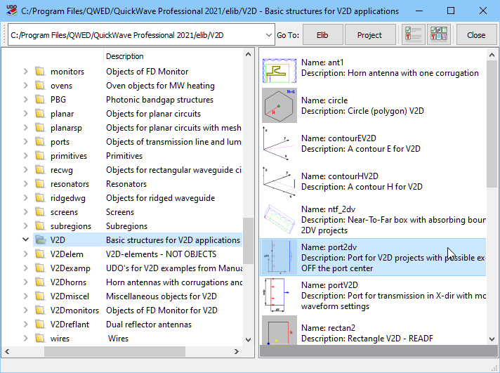
Fig. 3.2-15. V2D folder in the UDO library.

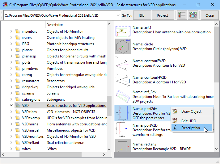
Fig. 3.2-16. Description option in UDO library.

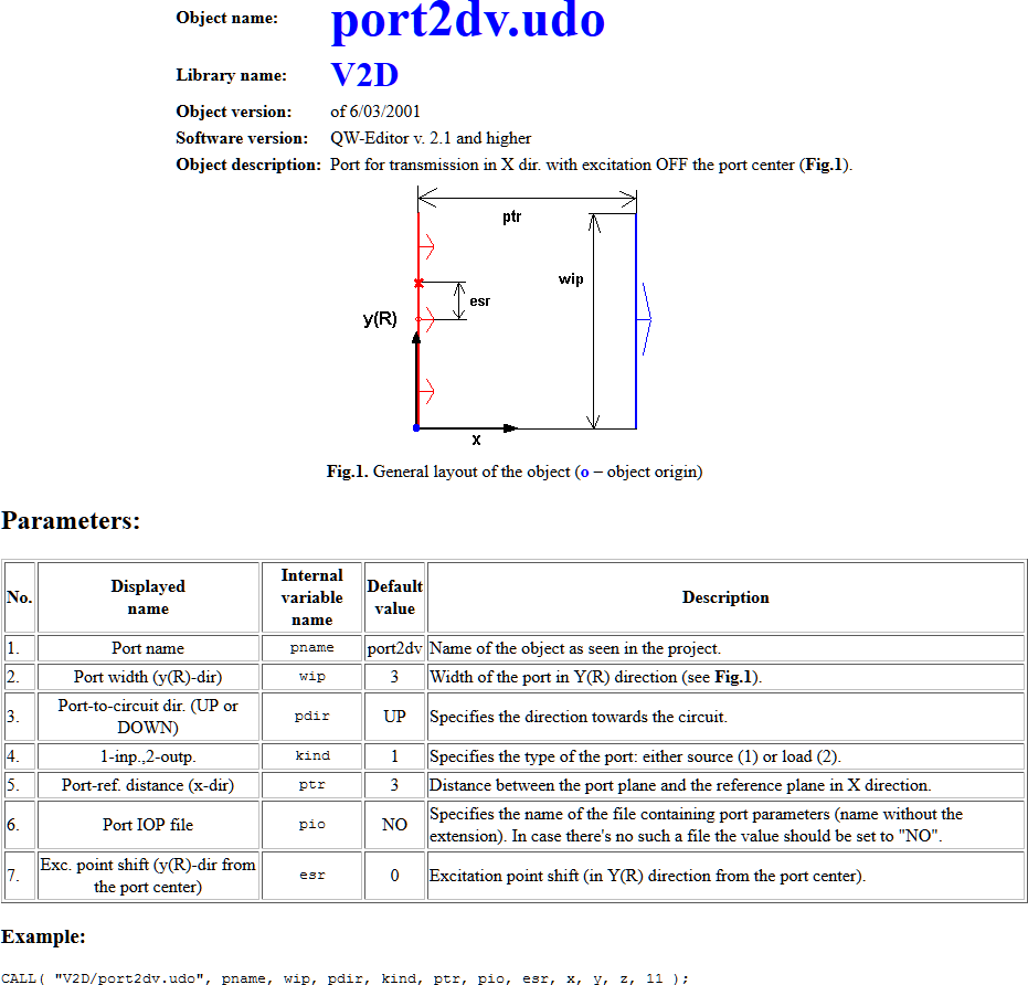
Fig. 3.2-17. Description of the port2dv object.

In this case the CALL command syntax is following:

CALL( "V2D/port2dv.udo", pname, wip, pdir, kind, ptr, pio, esr, x, y, z, 11 );

where:

pname – name of the object which will be seen in the project,

wip – width of the port in y (r) direction,

pdir – specifies the direction towards the circuit (UP or DOWN),

kind – specifies the type of the port: source (1), load (2),

ptr – distance between port plane and the reference plane in x direction,

pio – specifies the name of the *.iop file containing port parameters (name without the extension); NO if there is no such file,

esr – excitation point shift in y (r) direction from the centre

Fig. 3.2-18 shows the definition of the exciting port. Name of the port is source and its height is the same as the inner radius of the waveguide (ir). The source excites UP towards the circuit and since it is a source its type is 1. The reference plane (the plane at which the S parameters are calculated) is placed in a distance of half of the waveguide length from the port plane towards circuit (RD). We recommend that the reference plane is placed 4-5 FDTD cells from the port plane to assure accurate results of S parameters calculation (the reference plane position maybe later modified if, after setting the mesh parameters, it turns out that it is too close to port plane). We do not indicate any *.iop file with port parameters (NO) but it will be modified later, after setting the excitation parameters in QW-Editor. The excitation point has been moved by 0.3 of the inner radius of the waveguide (yexc), thus it will be placed at height of 0.8 of the inner radius of the waveguide. The exciting point has been moved close to the waveguide wall, where for mode TE11 longitudinal component of magnetic field (in QW-V2D it is H_x component) has its maximum. This component will be further used for exciting the antenna. If we liked to excite the antenna with other electromagnetic field component, we would need to place the exciting point in a place where this component gets maximum values.

The port is placed at the (0,0) point.

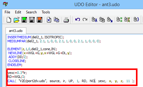
Fig. 3.2-18. Definition of the excitation port.

The last crucial element that needs to be defined in the UDO script is NTF box (together with absorbing box and magnetic symmetry plane). Here we will also use the NTF box available in the UDO library (see Fig. 3.2-19). According to the Description, when using this library object it is required to set the length (in X direction) and the radius of NTF and absorbing boxes. By default, the NTF box is placed in the centre of absorbing box, however, the position of NTF box may be shifted with respect to its default central position. This shift needs to be also defined. The NTF and absorbing boxes dimensions for considered dielectric antenna are defined in Fig. 3.2-20 and their values are given in Table 2. The ntf_2dv.udo inserts also a magnetic symmetry plane at the lower wall of the box.

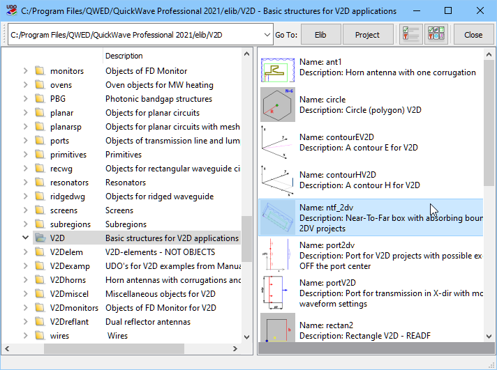
Fig. 3.2-19. V2D directory in elib UDO library.

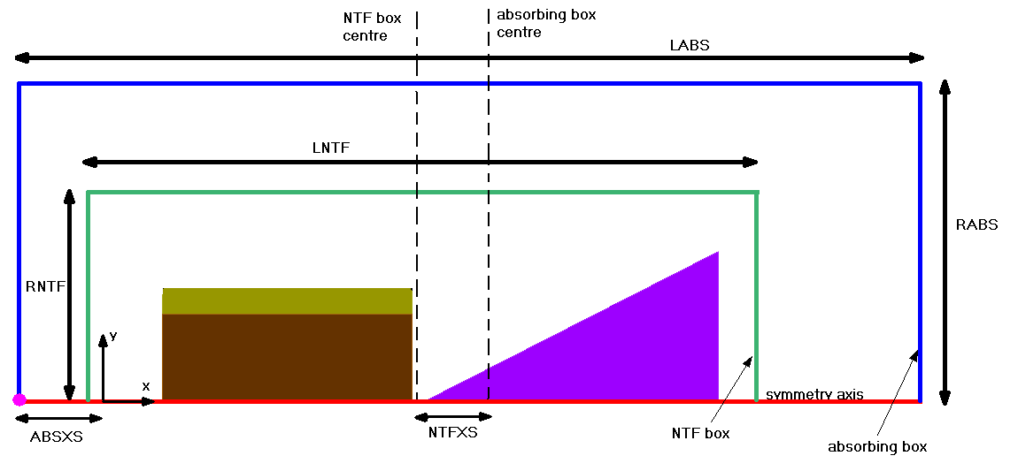
Fig. 3.2-20. NTF and absorbing boxes dimensions for dielectric antenna.

Table 2 NTF and absorbing boxes dimensions.

To be able to resize the NTF and absorbing boxes during the design process the above variables will be declared as UDO parameters. Thus we need to go back to UDO header and declare additional parameters using PAR command as given in Fig. 3.2-21.

When the parameters have been declared we may define the NTF box. The CALL command syntax available in the Description is as follows:

CALL( "V2D/ntf_2dv.udo", L, R, dntf, sntf, ntfxs, x, y, z, 9 );

where:

L – length of the absorbing box in X direction,

R – radius of the absorbing box,

dntf – length of the NTF box in X direction,

sntf – radius of the absorbing box

ntfxs – NTF box shift with respect to the central position in X direction.

We define NTF box in the UDO script as in Fig. 3.2-22 (green frame). It is worth noting that the absorbing box is shifted in X direction by the distance of ABSXS (-10 mm) from the (0,0) point.

At this point two hints regarding the NTF and absorbing boxes should be given:

1. NTF surface should be usually placed as close the object as possible provided that there is at least 3 FDTD cells distance. In case of dipoles radiating in free space, bigger distance can be required.

2. The distance between the NTF surface and absorbing boundary must be at least 3 FDTD cells.

The fact that the NTF and absorbing boxes dimensions have been declared as UDO parameters enables their easy resize if the above conditions are not obeyed after setting the mesh parameters in QW-Editor.

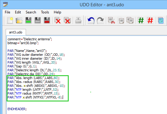
Fig. 3.2-21. UDO parameters list.

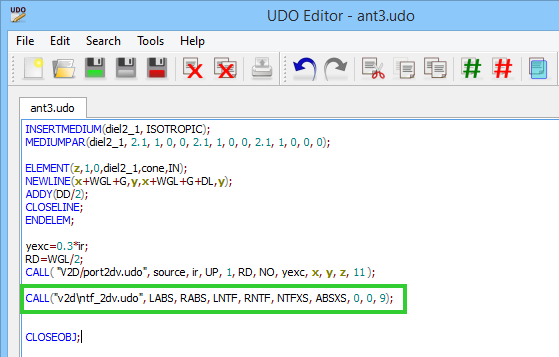
Fig. 3.2-22. Definition of the NTF box (with absorbing box).

This ends the UDO script creation process. We put the CLOSEOBJ command at the end of the UDO script and now we can proceed with simulation project (*.pro) preparation.