2.13.2   Contours E, H and combination of them

In the previous Section we have considered an example of electric field integration over a simple contour in a parallel plate line. Here we will present two more complicated and more practical examples, in which we will apply new features of the software. Namely, we will use integration of both electric and magnetic fields over specific contours and present the results of their ratio that can be interpreted as the characteristic impedance of a TEM transmission line.

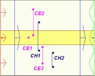
Let us open the ..\Various\Contours\tl0.pro example. We can see five defined contours. Three of them CE, CE2 and CE3 are the E-field integration contours, and two of them: CH1 and CH2 are the H-field integration contours. They are all presented in Fig. 2.13.2-1 where the QW-Editor displays in XY and YZ planes are supplemented by descriptions of the contours names. We can see that the problem concerns a TEM line (a shielded stripline) with the strip marked in yellow. Lower part of the line is filled with a substrate (light green). However, in the example tl0.pro we assume that the substrate has the same properties as air. This is in contrast to example tl1.pro where the substrate is made of FR4 of relative permittivity 3.8. The substrate has thickness of 20 mils.

Fig. 2.13.2-1 Contours considered in tl0.pro and tl1.pro examples.

The definition of the contours is specific for presentation of TEM and quasi-TEM line properties. CE1 and CE2 are different integration lines between the strip and ground. CE3 is a closed contour of E-field. One of H-field contours (CH1) makes a loop around the strip while the other provides the results of integration outside the strip. In the case of pure TEM wave we should have the following results:

- integration over contours CE3 and CH2 should give zero,

- results of integration over CE1 and CE2 should be equal,

- ratio of the results of integration over CE1 and CH1 (or CE2 and CH1) should not depend on frequency and be equal to the characteristic impedance of the considered TEM line.

Let us now run the example tl0.pro. There are four displays of results that should be opened by the user: CH2, CE3, CE1/CH1, and CE2/CH1,The first two of them open upon choosing consecutively CH2, CE3 results under  button in Results tab of QW-Simulator. The other stand for the combination results of E and H contours. The result window of one of them is presented in Fig. 2.13.2-2. It shows the result of integration over contours CE1, CH1 as well as their ratio – perfectly constant versus frequency. For the purpose of getting such display choose  under  button. The FD-Probing Postprocessings dialogue as in Fig. 2.13.2-3 appears. To obtain the window as presented in Fig. 2.13.2-2 we should choose the contours CE1 and CH1 (please use Ctrl+mouse click to pick up correct contours from the list). Then choose Combine Contours and click OK. The window as in Fig. 2.13.2-2 should be restored. The same operations should be performed to get CE2/CH2.

Each of the windows has a description of the displayed results in its status bar. Please verify that all the results are in a very good agreement with theoretical prediction of the TEM line properties presented above.

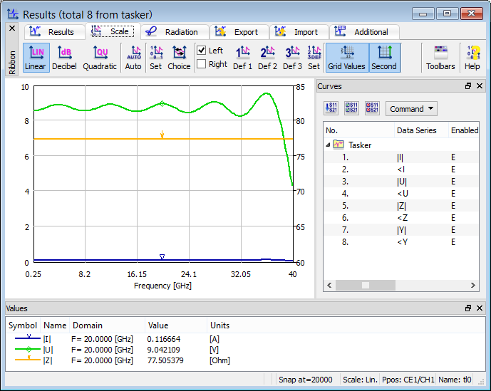
Fig. 2.13.2-2 Results of integration over contours CE1 and CH1 of tl0.pro example.

Now please run the second example: tl1.pro concerning a shielded microstrip on a dielectric substrate. Thus we consider a case of a quasi-TEM transmission line. The obtained results of simulation make it clear that this line can be considered as a TEM line only in a relatively narrow frequency band. In particular, the impedance calculated from contours CE1 and CH1 changes considerably as presented in Fig. 2.13.2-4.

Fig. 2.13.2-3 Postprocessing list dialogue in tl0.pro example.

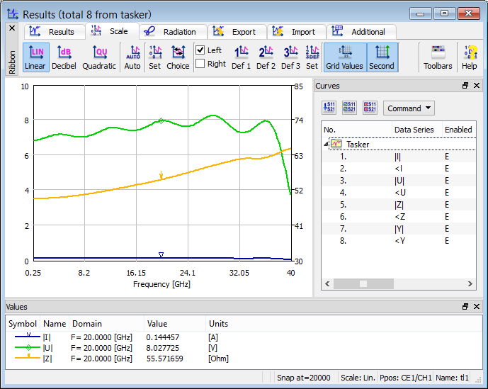
Fig. 2.13.2-4 Results of integration over contours CE1 and CH1 of tl1.pro example, with voltage and current assigned to the left scale and impedance assigned to the right scale.