2D propagation in dispersive material with Kerr and Raman nonlinearities
The present example considers 2D propagation in a dispersive material with Kerr and Raman nonlinearities.
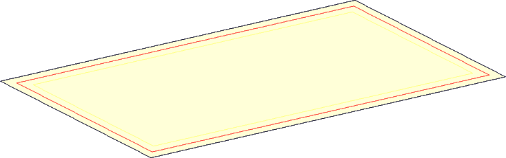
A two-dimensional line filled with a dispersive material.
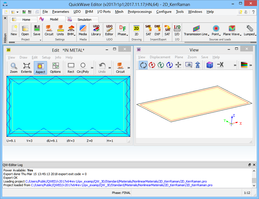
A two-dimensional line filled with a dispersive material project in QW-Editor.
The size of the scenario is 10 x 20 μm2.
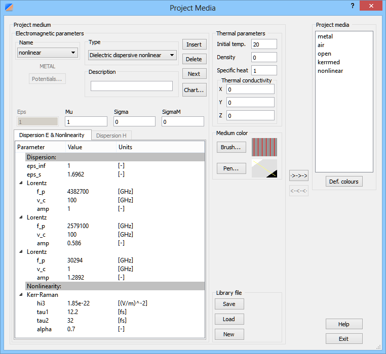
Simulation model considers propagation of a TM wave in a two-dimensional line filled with a dispersive material represented by the triple-pole Lorentz model which corresponds to the Sellmeier parameters given in Z. Lubin, J. H. Greene, and A. Taflove, "FDTD Computational Study of Ultra-Narrow TM Non-Paraxial Spatial Soliton Interactions", IEEE Microwave and Wireless Components Letters, vol. 21, no. 5, pp. 228-230, 2011.
The triple-pole Lorentz model is supplemented with third-order Kerr and Raman nonlinearities:
Parameters od the dispersive material given by Lorentz model supplemented with Kerr and Raman nonlinearities.
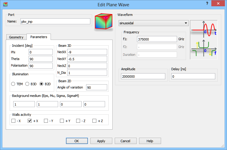
The two-dimensional line is excited with two free space incident waves (excitation is realised by two PLW boxes, marked red, situated at the same place and surrounded by absorbing exterior boundaries, marked as blue boxes). The 2D Gaussian beam (B2D option) is used for both excitations, however different values for X and Y neck centre are set. The excitation is towards +X direction (only +X chosen in Walls activity option).
First exciting wave settings.
Second exciting wave settings.
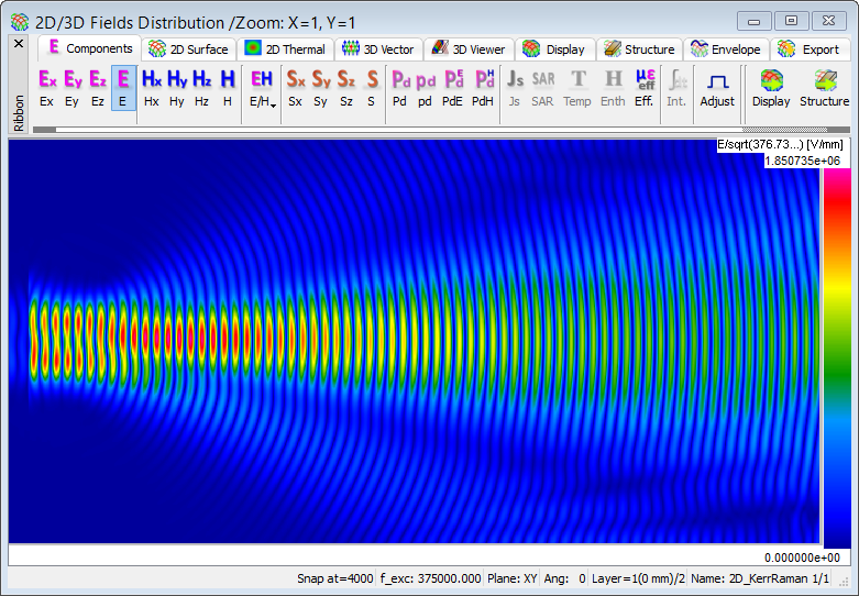
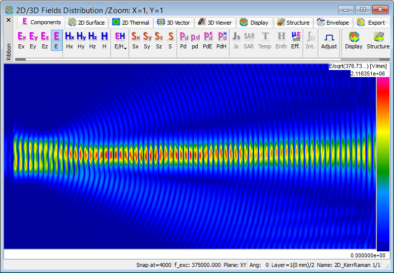
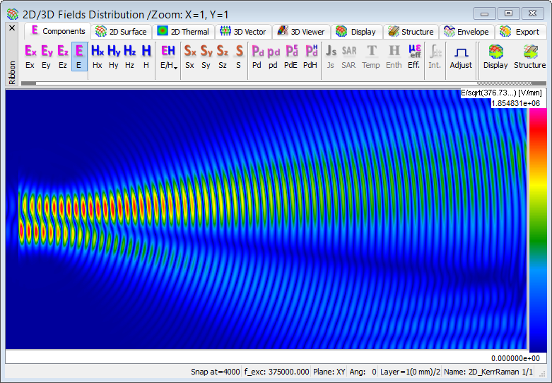
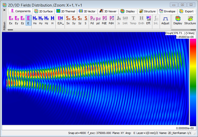
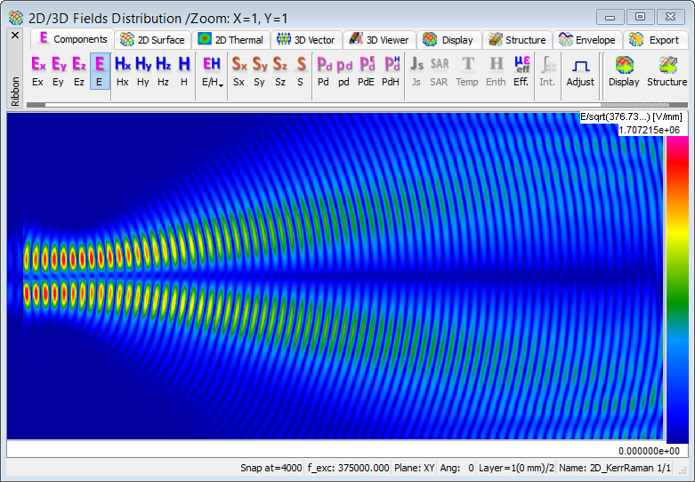
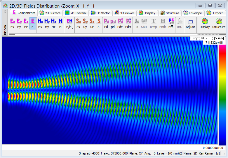
The structure is excited with different phase shifts between exciting pulses (excitation in phase, in quadrature, and out of phase) in and influence of the material nonlinearities is investigated. As a reference the same is investigated for a linear material. It can be seen that two pulses launched in phase merge into a single beam due to nonlinear effects. However, if the pulses are launched in quadrature, one soliton sucks off the energy of the neighbouring soliton. Eventually, antiphase driving of the two neighbouring pulses causes them to diverge from each other.
The total E field in linear (top) and nonlinear (bottom) regimes for two pulses, separated by 1.1 µm, launched in phase (Delay=0 ns).
The total E field in linear (top) and nonlinear (bottom) regimes for two pulses, separated by 1.1 µm, launched in quadrature (Delay=6.66667*10-7 ns).
The total E field in linear (top) and nonlinear (bottom) regimes for two pulses, separated by 1.1 µm, launched in antiphase (Delay=1.33333*10-6 ns).