4.1.2 The nonlinear model of QW-HFM
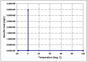
In principle, equation (4.1-1) can be applied to modelling of non-linear problems. However, in the vicinity of the phase-change temperature (which is e.g. 0ºC for water) rapid rise of the values of the fc function – specific heat – occurs in some media. An example specific heat versus temperature curve is shown in Fig. 4.1.1.1-1: specific heat of pork equals approximately 3 Jg-1C-1 in a broad temperature range, but increases by five orders in magnitude around the thawing point.
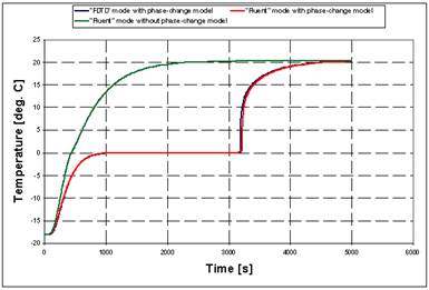
The figure Fig. 4.1.1.1-1 also contains a comparison of three curves showing temperature evolution in the centre of deeply frozen sample heated from outside through convection. The comparison has been provided in order to illustrate how using the phase-change model can affect computations. The curves obtained with the phase-change model (either the one implemented internally in the QW-HFM or in Fluent) differ to a great extent from the results calculated without taking the phase-change effect into consideration. When the phase-change occurs, the temperature at the melting point is kept at a constant level until the heat absorbed from the boundary condition becomes equal to the latent heat of the phase-change. Working with a constant specific heat value taken below the thawing point means ignoring the latent heat, and deteriorating accuracy of computations.
Fig. 4.1.1.1-1 a) The specific heat vs. temperature curve for medium “pork”; b) simulation of thawing of a sample made of “pork” performed with- and without phase-change model (blue line – curve obtained with QW‑HFM module working in FDTD mode with phase-change model; red line – curve obtained in Fluent mode with phase-change model; green line – curve obtained in Fluent mode without phase-change model).
To simulate scenarios involving media with phase-change (an effect occurring in thawing of frozen food products), equation (4.1-1) should be reformulated. The alternative formulation of the heat transfer equation, which can be directly applied to problems with phase-change media, is shown below.
![]()
(4.1.1.1-1)
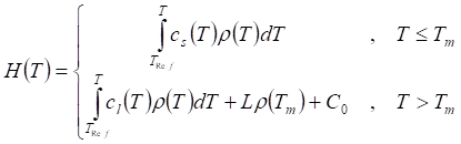
where T is the temperature field, k(T) is thermal conductivity of the medium (in general it can be dependent on the current temperature) and H is the enthalpy field (given in J/cm3) defined in the following way:
(4.1.1.1-2)
where:
TRef - arbitrarily chosen reference temperature defined (typically it is the initial temperature which makes it possible to avoid negative values of the enthalpy field);
cs(T) - specific heat of the medium in the solid phase (in general case it is temperature dependent);
cl(T) - specific heat of the medium in the liquid phase (in general case it is temperature dependent);
L ![]() - latent heat of phase change;
- latent heat of phase change;
r(T) - density of the medium (in general case it is temperature dependent);
Tm ![]() - the temperature of melting;
- the temperature of melting;
C0 ![]() - a constant defined as shown below:
- a constant defined as shown below:
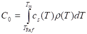
(4.1.1.1-3)
With this formulation one avoids explicitly using specific heat values in computations, replacing them with integral functions, which are still non-differentiable at the temperature of melting but are far easier to handle than delta-like specific heat vs. temperature curves. This approach does not limit users’ ability to properly define media involved in the analysis by providing their descriptions in form of the H=f(T) function containing also the latent heat value crucial to accurately simulate thawing, melting and solidification processes.
The nonlinear heat transfer model, with the phase change effect, is activated by UseNonlinearModel option checked in Preferences dialogue of QW-Simulator in HFM INI tab or by setting UseNonlinearModel=true in the initialisation file (hfm.ini in the /envir installation subdirectory). By default the nonlinear model is turned off. More information about options available in the initialisation file can be found in The initialisation file.
The computations are then performed directly on the enthalpy field, which means that it is the enthalpy fields instead of temperature which is repetitively updated every iteration Dt. The current temperature field needed in (4.1.1.1-1) for calculating temperature gradient is extracted from the *.pmo file data. The *.pmo file contains the definition of the H = f(T) function (the Temperature column with corresponding values in the Enthalpy column). Using the inverse function it is possible to estimate the temperature based on the current enthalpy field.
The discretised equation has the following form:
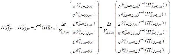
(4.1.1.1-4)
QW-HFM working in the FDTD mode with nonlinear model requires Temperature, Enthalpy and Ka (or Kx, Ky, Kz) columns in media *pmo files. Density and SpecHeat listed in these files are ignored, as their product is extracted from the H=f(T) function. When QW-HFM is activated from QW-BHM, media parameters defined in *pmo files are interpolated at the temperature read from *.hfe. They will be modified in the course of thermal simulation following the current value of the enthalpy field, the behaviour of the H=f(T) function (in case of specific heat and density) and the k=f(T) function (in case of thermal conductivity). Without this feature modelling of phase-change problems would be inaccurate. This does not mean, however, that no care should be taken while choosing the step Dt. QW-HFM is never used as a stand-alone application, but rather as a part of a coupled electromagnetic-thermal model. Thus, media properties change not only as a result of heat transfer effect, but especially due to electromagnetic power dissipation. Maintaining the step Dt small enough ensures that thermal media parameters do not change too much, which leads to an improved accuracy.
Due to the input data – especially the H=f(T) function – the analysed problem can become strongly nonlinear. Because of this the length of the time-step is adjusted every iteration maintaining stability of the method and ensuring high accuracy of computations. It is also the reason why the analysis of problems with extremely long heating times may last longer as compared to cases where the phase change model is not used.