2.2.2    Display Charts

The results curves can be displayed in various coordinates:

·       XY

·       Polar

·       Smith

·       Rieke

2.2.2.1   XY

The  button in Results tab and Coordinates->XY command from main menu or context menu switch the display to XY chart that allows displaying the results in orthogonal XY coordinates (Cartesian coordinates).

XY chart can be used for displaying SWR and GD results. The Y scale grid contains by default the following grid positions: 1.2, 1.5, 2, 3, 4, 5, 7, 10 and 20. The Y scale grid can be controlled by gridlines.gr3 file placed in the project directory (see Rieke chapter for more information).

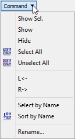
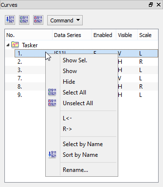
The Values pane contains information about visible curves such as name, domain, and value under active cursor and other parameters in separated columns, which can be chosen in Select Column dialogue.

2.2.2.2   Polar

The  button in Results tab and Coordinates->Polar command from main menu or context menu switch the display to Polar chart that allows displaying the results in polar coordinates.

The Values pane contains information about visible curves such as name, domain, and value under active cursor and other parameters in separated columns, which can be chosen in Select Column dialogue.

2.2.2.3   Smith

The  button in Results tab and Coordinates->Smith command from main menu or context menu switch the display to Smith chart. Smith chart (Alt+M) is relevant only for the display of S-Parameters results. It temporarily changes the window scale to Linear (Decibel or Quadratic scale will be restored when coordinates change back to XY or Polar).

The Values pane contains information about visible curves such as name, domain, and value under active cursor and other parameters in separated columns, which can be chosen in Select Column dialogue.

2.2.2.4   Rieke

The  button in Results tab and Coordinates->Smith command from main menu or context menu switch the display to Rieke chart when SWR & GD option is switched on.

Rieke chart is available for Standing Wave Ratio and Group Delay results.

The rings are placed by default at 1.2 1.5 2.0 3.0 4.0 5.0 7.0 10 20 but can be placed differently through a gridlines.gr3 file in the project directory. Radial phase lines are placed by default at every 0.05 wavelength and can also be spaced differently through a gridlines.gr3 file in the project directory.

In the Rieke chart, the quantity plotted is equal to SWR in magnitude but with the phase of S₁₁. In the radial direction, the Rieke chart spans the whole range of reflection values, from |S₁₁|=0 (SWR=1) at the chart centre to |S₁₁|=1 (SWR-->inf) at the chart outermost circumference. Scaling in the radial direction is linear in terms of |S₁₁|, gridding is shown in terms of the SWR values. Hence the value in the chart centre is 1 and consecutive rings are placed by default at 1.2 1.5 2.0 3.0 4.0 5.0 7.0 10 20. Different rings, at arbitrary positions, can be enforced by the user through a gridlines.gr3 file in the project directory. Radial phase lines in the Rieke chart are placed by default at every 0.05 wavelength. Different angular spacing can also be obtained through a gridlines.gr3 file in the project directory.

Example 1: gridlines.gr3 which produces gridding identical to default settings

!YSWRGridLines

1.2 1.5 2.0 3.0 4.0 5.0 7.0 10 20

!XSWRGridLines

0.05

Note that gridlines.gr3 file, if available in the project directory, also controls the Y scale gridding in the XY chart when the SWR&GD option is switched on.

The Values pane contains information about visible curves such as name, domain, and value under active cursor and other parameters in separated columns, which can be chosen in Select Column dialogue.