2.2.8      Modal templates in inhomogeneous guides

The example of dielectric waveguide coupler can serve to look more closely at the mode templates in inhomogeneous guides. First let us try to recalculate the example including additional ports defined on higher modes. Please consider the project ..\PassiveComponents\Dcoupler\dcoup2.pro prepared using ..\examples\dcoup2.udo. It differs from the previously considered one by three additional ports 5-7 defined in the same place as ports 1-3 but at higher dielectric waveguide modes. Let us run dcoup2.pro. We can see that at the beginning of the simulation QW-Simulator calculates templates for the first four ports (inp, out1, out2, out3) and then continues for three other ports (inbis, ou1bis, ou2bis). The parameters for these ports have been defined in a way that the higher mode templates are generated for them. Thus different effective permittivity has been set in port settings dialogue and the excitation point for template generation has been moved away from the centre of the port to excite also modes, which have zero field in the centre. Let us wait until the Simulator Log displays the sequence of messages:

for port inbis and then press  to see the template field distribution as presented in Fig. 2.2.8-1. We can see that now the mode template is that of the second mode in the dielectric waveguide. Contrary to the dominant one presented in Fig. 2.2.7-2it has an odd symmetry with respect to the centre of the guide.

Fig. 2.2.8-1 E_z filed distribution across a dielectric waveguide port inbis of dcoup2.pro.

Fig. 2.2.8-2 Results of analysis of S-parameters of dcoup2.pro in 80-120 GHz band.

Now let us continue the simulation of the example dcoup2.pro. After about 1500 iterations of the 3-D simulation please press  button to open Resultswindow to see the S-Parameters versus frequency. Now using Config dialogue we can choose the characteristics S11...S71 to be displayed as presented in Fig. 2.2.8-2. We can see there how big the reflection at the higher mode (S51) and transmissions at these modes to other ports (S61, S71) are. We can see that none of the three is very significant and this explains only slight improvement in the power balance at 100 GHz (from –1.33 dB in Fig. 2.2.7-3to –0.941 dB in Fig. 2.2.8-2). Still almost 1 dB is lost to radiation or transformation to other modes.

Let us also have a look at the propagation constants of both modes. Open another Resultswindow by pressing  button. Gam2 and Gam6 curves will be displayed. We obtain the picture of Fig. 2.2.8-3. It illustrates two features of inhomogeneously filled waveguide modes:

- it is difficult to predict analytically the dispersion characteristics of them,

- propagation constants of different modes may be relatively close to each other.

Fig. 2.2.8-3 Results of analysis of Gam2 and Gam6 of dcoup2.pro in 80-120 GHz band.

The above features make the process of template generation for dielectric waveguides not so straightforward as for the rectangular or circular air-filled guides. Here we should assume that after introducing a new shape of the waveguide or a new frequency band, the proper choice of parameters needed for automatic template generation must be proceeded by some experiments with manual template generation (as explained in First insight template generation and Septum polariser as a six port with higher-order waveguide modes). Please experiment with the manual template generation using the test project ..\PassiveComponents\Dcoupler\dcouptest.pro. This project contains just a section of a dielectric waveguide (the same as one used in the previous projects) with the input port on one side and an absorbing port on the other side.

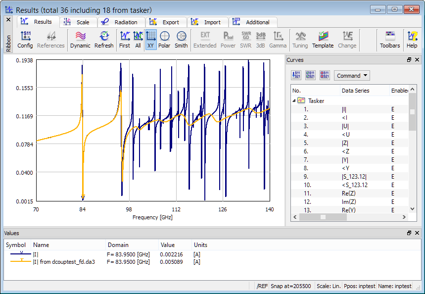
Fig. 2.2.8-4 Template mode detection curves of dcouptest.pro in 70-140 GHz band with (orange) and without (blue) the top absorption.

Please run dcouptest.pro and open Resultswindow by pressing  button to see the display of the template mode detection curves. After a sufficient number of iterations of this 2-D simulation we obtain the display as represented by the orange curve in Fig. 2.2.8-4. We can see that there are two resonances in the band of interest. They correspond to the modes we have already considered in this and previous Sections. However it is important to note that such a result has been obtained with the absorbing boundary assumed at the top of the box. This absorption is taken into account during the template generation and attenuates the possible “box modes” that could be generated if there are electric boundary conditions around the port.

To see what would happen without the absorbing boundary please invoke Select Element dialogue and on the list of elements delete the absorbing element named – mur2. Then rerun the project. As a result you will obtain the display represented by the blue curve in Fig. 2.2.8-4. It indicates more than a dozen of different modes. Most of them are the “box modes” or in other words the rectangular waveguide modes with the electromagnetic fields not confined to the dielectric core of the waveguide. Such modes are not of interest in our application and thus it is correct that they are eliminated by the top absorption. The images of Fig. 2.2.8-4underline the importance of the absorption in the search for the dielectric waveguide modes. Without an absorbing side it is very difficult to distinguish which of the modes are those really guided in the dielectric core.