2.3.8      Near-to-Far transformation at the fixed angle

There is another post-processing allowing the far field radiation analysis, called NTF at Fixed Angle (NTFFA). Sometimes, especially in radar applications, our aim is to control the shape of the pulse as well as its spectrum in the far zone at the particular direction from the transmitting antenna - rather than the radiation characteristic over a range of angles, at a few fixed frequencies. This would be very time-consuming to obtain with NTF transform described in the Rectangular waveguide horn in open space since it performs a Fourier transform of the electromagnetic field at the NTF box followed by near-to-far transformation in the frequency domain. To the contrary, NTF at Fixed Angle performs the near-to-far transformation in the time domain, directly from the time-domain fields at the NTF box. The far-field results is then Fourier-transformed.

Consider the horn1_ntffa.pro example to clarify the main features of this new post-processing.

Like in horn1.pro, the antenna is excited with the TE10 mode within the 18 – 30 GHz band (see Fig. 2.3.1-2). We want to observe the radiated pulse in the far zone exactly in front of the antenna. We use one NTF box to define both NTF and NTFFA post-processings which may work simultaneously. Invoke Near To Far and NTF Fixed Angle dialogue (see Fig. 2.3.8-1) and focus on the NTF Fixed Angle dialogue. In the first line we specify which NTF walls should take part in the calculation. In the second line we set the spectrum of the Fourier transform to be performed on the far zone signal. In the last line we specify all the directions of interest in the following manner:

φ₁ q₁; φ₂ q₂; …

where φ and q  are the azimuthal and elevation angles (in degrees) of the spherical coordinate system with the Z-axis as a reference (q  is measured from the Z-axis and φ is measured from the X-axis in the XY-plane).

Fig. 2.3.8-1 Near To Far and NTF Fixed Angle dialogues in the example horn1_ntffa.pro.

Let us launch the simulation without run with  button. Press  button in Run tab of QW-Simulator twice to get through the input template computation to the beginning of the 3D simulation. When QW‑Simulator suspends at this point, invoke the 1D Fields window by pressing  button in 1D Fields tab.

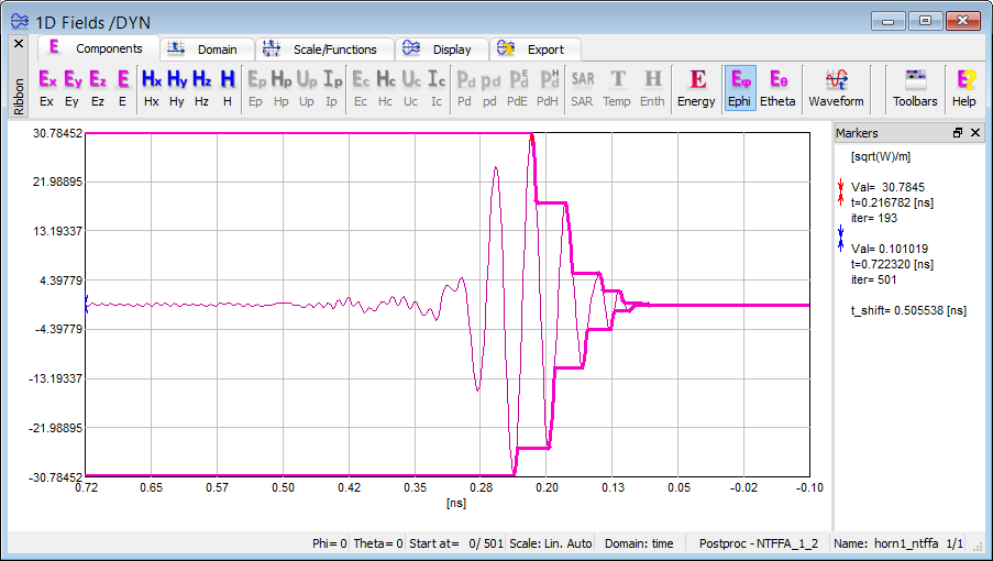
Fig. 2.3.8-2 1D Fields window in the example horn1_ntffa.pro.

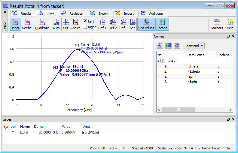
Fig. 2.3.8-3 Antenna Fixed Angle Results window in the example horn1_ntffa.pro.

Start the 3D simulation with  button and watch the 1D Fields window. It will be showing the pulse in the far zone, as a function of time (Fig. 2.3.8-2). When the pulse eventually fades away, we may look at its Fourier transform in Results window invoked with  button from Results tab as in Fig. 2.3.8-3. Both instantaneous far field and its Fourier transform calculated with NTFFA are in sqrt(W)/m units, similarly like in NTF Fields at 1m. Therefore, we may directly compare the NTF and NTFFA results.

Let us then invoke NTF results by pressing  button in 2D Radiation Pattern section of Results tab in QW-Simulator and look at the peak value of the main lobe in Fields at 1m scale (Fig. 2.3.8-4). For both 20 and 25 GHz frequencies discrepancy is about 1% what apparently results from different approaches incorporated in both post-processings.

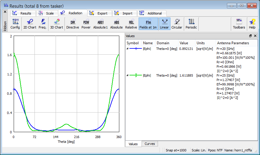
Fig. 2.3.8-4 2D radiation pattern results in the example horn1_ntffa.pro.