2.5.1      Dielectric resonator

A dielectric resonator example has been prepared and saved in ..\Resonators\Dielres\dielres1.pro and ..|Resonators\Dielres\dielres2.pro files. Both files describe the same structure and have been created from the same examples\dielres.udo parameterised object. One of this object‘s parameters is the name of the *.iop file wherefrom the source port parameters are to be read. In the two examples two different files: ex_pulse.iop and ex_sin.iop have been specified, respectively. As a consequence, dielres1.pro is run with pulse excitation and FD-Probing post-processing, producing eigenfrequencies of the structure while dielres2.pro is run with sinusoidal excitation producing modal field patterns of one of the modes.

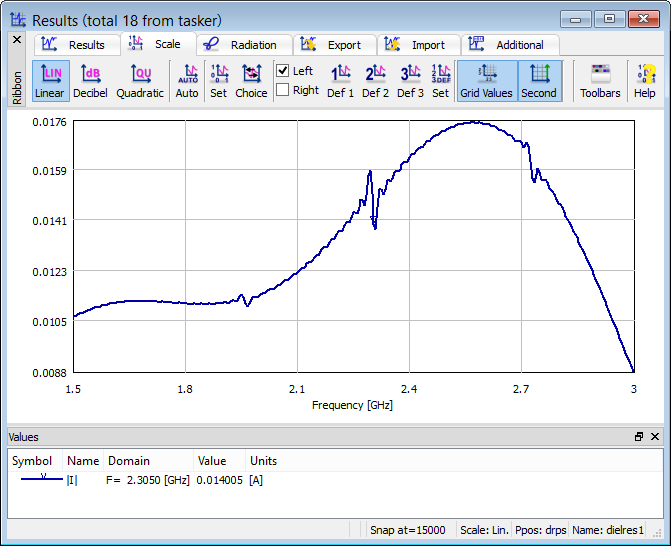
Fig. 2.5.1-1 Fourier transform of current flowing between the point source and the resonator, with minima indicating resonant frequencies (dielres1.pro example).

When analysing dielres1.pro, we open Results window with FD-Probing results by pressing  button in Results tab of QW-Simulator. We obtain the curve of Fig. 2.5.1-1. It indicates resonant frequencies at 1.965, 2.305 and 2.730 GHz. In the dielres1.pro example two 2D FD Monitors have been included to enable obtaining 2D Fourier transforms of time-domain fields at each of those frequencies. Sample results are shown in Fig. 2.5.1-2 and Fig. 2.5.1-3 and they are obtained by pressing four times the  button in Monitor tab of QW-Simulator.

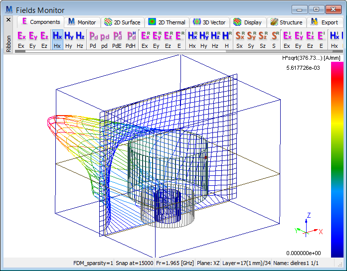
Fig. 2.5.1-2 Fourier transform of Hx field in horizontal and vertical monitoring planes set in dielres1.pro example, at two resonant frequencies, obtained from a single simulation.

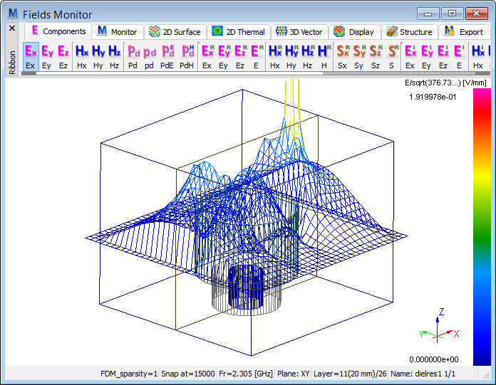
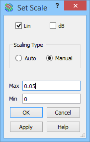
Fig. 2.5.1-3 Fourier transform of Ex field in horizontal monitoring plane set in dielres1.pro example, at 2.305 GHz;  upper – automatic scale, lower left – manual scale restricted to 0.05, lower right – Set Scale dialogue accessible by double-clicking over the scale colour bar.

When looking at the Ex field in the plane including the Ex excitation point, we get the picture of Fig. 2.5.1-3 (left) dominated by the potential spike due to divergence at the source. We may cut off this spike by setting a restricted manual scale. This is done by double-clicking over the scale colour bar, and making proper adjustment in the Set Scale dialogue shown in Fig. 2.5.1-3.

Please run the two examples and try to apply the experience in application of S-parameters and field displays gained from examples of Waveguide-to-coax transition.