2.11.4 One dipole near electric wall
In terms of the shape of radiation pattern, the circuit comprising two Ez dipoles mutually shifted along the X-axis and excited out-of-phase is equivalent to the circuit occupying only half of the space, with one dipole and an electric symmetry plane perpendicular to the X-axis. The analysis with the symmetry plane will be advantageous since it permits to reduce the memory requirements and computing time by half.
The simulation scenario with one dipole and electric symmetry plane has been prepared in the ..|Antennas\Dipole\1dipe.pro. The user may wish to prepare the project by his own by modification of 2dip.pro example as described in below steps. Note that the symmetry conditions must be taken into account in the calculation of radiation patterns. Thus, what we need is an NTF box “instructed” about the electric symmetry along the X-axis. Let us first summarise basic principles about NTF calculations with symmetry planes in QW-3D:
a) The circuit must be situated in the positive X- and/or Y- and/or Z-direction from the symmetry planes.
b) The symmetry plane must coincide with mesh boundary (the meshed region cannot extend beyond the symmetry plane). Remember that mesh boundaries are defined in Mesh Parameters dialogue. It is possible to mesh only a subregion of the circuit, but no ports may extend beyond this meshed subregion.
c) An appropriate wall of the NTF box must coincide with the symmetry plane.
The best way to produce a proper NTF box is to modify our ntf.udo object:
1. Please press the ![]() button in 2D Window. The Select Object dialogue shows only one object: ntf.
button in 2D Window. The Select Object dialogue shows only one object: ntf.
2. Select this object by double-clicking the left mouse button.
3. You will see the dialogue with the last introduced object parameters.
4. Do not be surprised that the name of the dialogue starts with Add Object. Internally in the QW-3D software, object modification is accomplished by cancelling the object in question, and then defining it again (with the last set of parameters suggested in the dialogue). Please make the following changes in parameters:
¨ X plane E (which stands for electric wall in the X-direction)
¨ AbsLength 24 (reducing the space by half along the X-axis)
¨ NTFLength 16 (also reduced by half along the X-axis)
¨ Origin X 24 (to locate the symmetry plane at its natural location x=20)
¨ Press Draw to exit the dialogue and draw the modified object.
5. Now the dipole outside the NTF box should be deleted. Press ![]() button, press left mouse button over point2 in the dialogue, press Delete button, press Close.
button, press left mouse button over point2 in the dialogue, press Delete button, press Close.
7. Note that the correct settings for post-processing and dipole excitation are inherited after 2dip.pro (you may enter the two dialogues to verify this).
Press ![]() to start the analysis. After a few hundred of iterations press
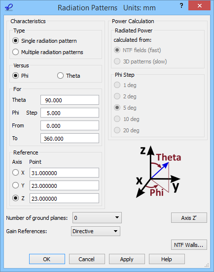
to start the analysis. After a few hundred of iterations press ![]() button in Results tab of QW-Simulator. Radiation Patterns dialogue will appear. The parameters for radiation pattern calculations should be as in the picture below. It now includes an additional Number of ground planes field. This is because QW-Simulator is calculating radiation patterns with X-symmetry, which may correspond to either of the two physical cases:
button in Results tab of QW-Simulator. Radiation Patterns dialogue will appear. The parameters for radiation pattern calculations should be as in the picture below. It now includes an additional Number of ground planes field. This is because QW-Simulator is calculating radiation patterns with X-symmetry, which may correspond to either of the two physical cases:
- two radiating dipoles, which is our case,
- one physical dipole radiating over an infinite ground plane.
Power radiated in the directions of phiÎ[(0°, 90°) È (270°, 360°)] is the same in the case of one and two dipoles. In the case of one dipole, there is no physical radiation for phiÎ(90°, 270°), but results with X-symmetry present a virtual mirror image of the physical half of the radiation pattern. Therefore, in the case of two dipoles and symmetry, the whole radiated power integrated by the software (in the physical and mirror half-space) should be taken as a reference for efficiency and gain calculations. In the case of one dipole and one physical ground plane, only the power in the physical half-space (or, in other words, half of power integrated over the whole space) should be taken as a reference power for efficiency and gain calculations.
Make the settings as below and press OK in the dialogue.
The characteristic at 6.25 GHz should be the same as in the previous ‘out-of phase’ experiment. To verify this press ![]() button in Import tab of Results window and choose previously saved resout.da3.. (Remember that the amplitude characteristic at 6.25 GHz is the first in this file, so it is displayed as desired). Now press
button in Import tab of Results window and choose previously saved resout.da3.. (Remember that the amplitude characteristic at 6.25 GHz is the first in this file, so it is displayed as desired). Now press ![]() button in Scale tab to obtain the following quadratic (power) scale result:
button in Scale tab to obtain the following quadratic (power) scale result:
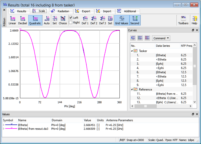
The blue (presently calculated) and magenta (reference) curves practically coincide. You may check that upon setting Number of ground planes =1 the two curves would differ by a factor of two.