2.11.5 One dipole near magnetic wall
The original circuit comprising two Ezdipoles mutually shifted along the X-axis and excited in-phase is physically equivalent to the circuit occupying only half of the space, with one dipole and a magnetic symmetry plane perpendicular to the X-axis.
Please open a ready to use ..\Antennas\Dipoles\1dipm.pro example with one dipole and magnetic symmetry plane or modify the 1dipe.pro project in the following way:
1. Please press the ![]() button in 2D Window. The Select Object dialogue shows only one object: 1. ntf.
button in 2D Window. The Select Object dialogue shows only one object: 1. ntf.
2. Select this object by double-clicking the left mouse button.
3. You will see the dialogue with the last introduced object parameters.
4. Please make one change in parameters:
¨ X plane M (which stands for magnetic wall in the X-direction)
¨ Press Draw to exit the dialogue and draw the modified object.
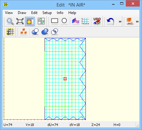
5. Note that the meshing of the circuit has changed. In our previous experiments, we had a line of cell edges (‘electric line’) for x=24 mm. Now magnetic boundary forces for x=24 mm a line of cell centres (‘magnetic line’). An important consequence of this change of meshing is that point1 no longer falls at the cell corner (where the desired Ez field component is not available). Thus the actual point of Ez excitation is offset from the original position:

6. To correct this, we can force a mesh snapping plane (‘electric line’) through point1, that is, at x=36 mm. Please click ![]() button in 2D Window. In the Special Planes and Boundaries dialogue electric and Orientation: X are the defaults, so just print 36 in Position field and press Insert and then Cancel to close the dialogue. Note that the meshing has changed and the Ez exciting field coincides with point1:
button in 2D Window. In the Special Planes and Boundaries dialogue electric and Orientation: X are the defaults, so just print 36 in Position field and press Insert and then Cancel to close the dialogue. Note that the meshing has changed and the Ez exciting field coincides with point1:
8. Note that the correct settings for post-processing and dipole excitation settings are inherited after 1dipe.pro (you may enter the two dialogues to verify this).
Press ![]() to start the analysis. After a few hundred of iterations press
to start the analysis. After a few hundred of iterations press ![]() button in Results tab of QW-Simulator. In the Radiation Patterns dialogue make the settings as in 1dipe.pro and then OK in the dialogue.
button in Results tab of QW-Simulator. In the Radiation Patterns dialogue make the settings as in 1dipe.pro and then OK in the dialogue.
The characteristics at both 6.25 GHz and 12.5 GHz should be the same as the corresponding characteristics in the previous ‘in-phase’ experiment. We shall verify this for 6.25 GHz: press ![]() button in Import tab of Results window and choose previously saved resin.da3. Now open Config dialogue and on the list select (by a left mouse click) item 1 (|Etheta| for the current simulation) and item 11 (|Etheta| from the resin.da3 file) and press ShowSel. In the linear automatic scale you should see the picture as below.
button in Import tab of Results window and choose previously saved resin.da3. Now open Config dialogue and on the list select (by a left mouse click) item 1 (|Etheta| for the current simulation) and item 11 (|Etheta| from the resin.da3 file) and press ShowSel. In the linear automatic scale you should see the picture as below.
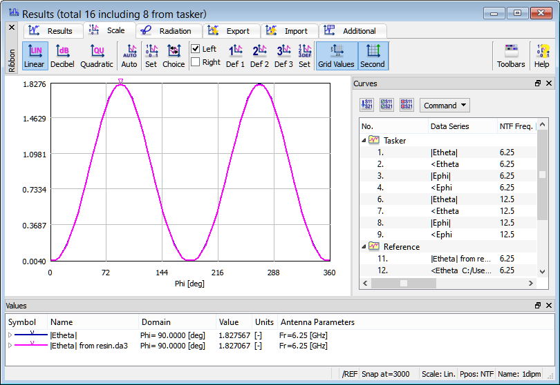
The two curves almost coincide, but there is a small visible discrepancy. In particular, the present example produces gain 1.827567 at 90 deg while the original 2dip.pro produced 1.827067. This is due to the difference of discretisation in these two projects. In 1dipm.pro we have 6.5 FDTD cells between x=24 mm and x=36 mm while in 2dip.pro - 7 cells. Let us return to the 2dip.pro project, and modify it by forcing a line of cell centres through x=24 mm and lines of cell edges at x=36 mm and x=12 mm.
Open the ..\Antennas\Dipoles\2dipm.pro example, where the magnetic mesh snapping plane has been introduced at X=24 thus where the magnetic symmetry plane is placed in 1dipm.pro.
Look at the meshing, analogous to the 1dipm.pro.

Please run the 2dipm.pro projectand compare the results with 2dip.pro and 1dipm.pro. In particular, please note that after 3000 iterations, 2dipm.pro produces gain 1.827588 at 90 deg.