2.7.1      A basic time domain reflectometry (TDR) example

Let us note that although QW-3D is a time-domain software, most of the post-processing functions discussed up to now have been concerned with the parameters extracted in the frequency domain (like S-matrices) or at some chosen frequencies (like radiation patterns). However, with fast advances of digital electronics in microwave frequency band there is a growing interest in the possibility to watch signals directly in the time domain like it is done in a measurement technique called Time Domain Reflectometry (TDR).

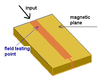
Fig. 2.7.1-1 The structure considered in the example tdr1.pro.

TDR-like signals can be extracted directly from QW-3D simulations. We will explain such a possibility using a simple example ..\Various\Tdr\ tdr1.pro. tdr1.pro has been drawn using especially prepared examples\tdr1.udo, which is a simple script composed entirely of calls to other objects available in standard QW-3D libraries. It contains a strip-line structure shown in Fig. 2.7.1-1. Actually, we are considering a lower half of the structure assuming a magnetic symmetry plane. Substrate is a 6 mm thick teflon. The input strip is 1 mm thick, 3.5 mm wide, and 32 mm long. It is terminated by a grounded strip of width 0.5 mm. During the simulation the structure will be excited by a step pulse and we will be considering E_z and H_y fields below the strip, at the point situated 3.36 mm from the input and thus 28.64 mm from the end of the wide strip.

Before running the example let us take a look at the Edit Transmission Line Port dialogue presented in Fig. 2.7.1-2. We have chosen a pulse waveform: step with finite rise time dt=1/f2 with f2=50 GHz. Let us justify this choice. In the considered project we use the cell size of 0.4 mm. For correct FDTD analysis the cell size should not be bigger than 0.1 of the wavelength. At 50 GHz the wavelength is 6 mm in air and about 4.2 mm in teflon. Thus with this FDTD mesh we should avoid exciting the circuit at the frequencies significantly higher than 50 GHz. It can be done by introducing a finite rise-time of the pulse as indicated above.

Now we press  button in Simulation tab of QW-Editor and then Create  button in Run tab of QW-Simulator (see Step by step simulation execution). QW-Simulator has been prepared for analysis but suspended before calculating the input port template. We are interested in watching the 3D analysis from the first iteration. Thus we press now Next Task  button. The software prepares the input port template and suspends its operation again. Let us note that it has calculated the input line impedance as 98.35 W. Actually this is the impedance of one half of the line and thus the entire line would have the impedance of 49.175 W.

We can now use invoke Test Mesh  window to choose a particular position of a cell where we want to watch the field changes. For that purpose press  button in Mesh tab of QW-Simulator to invoke Test Mesh window together with XYZ… dialogue delivering exact coordinates of a particular point, in millimetres. The Test Mesh window displays a correct FDTD layer (7^th) and we can check that the desired point x=3.36 mm, y=10 mm, z=-1.03 mm is included in the FDTD cell of indexes (011,028).

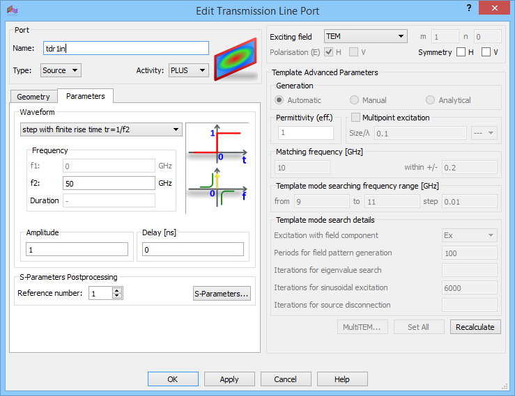
Fig. 2.7.1-2 The input port parameters for the example tdr1.pro. 

Now let us invoke 1D Fields window using  button from 1D Fields tab of QW-Simulator. The invoked window should remain the correct settings but let us discuss them here. The chosen field component is E_z. We click over  button in Domain tab. In the appearing Position & Parameters dialogue (Fig. 2.7.1-3) we are supposed to choose a digital position of the cell in X, Y and Z direction. The indexes (11,28,7), which as we have shown corresponds to the actual position of x=3.36 mm, y=10 mm, z=-1.03 mm, has been set. We can also choose the number of samples to be watched and the number of samples to be saved on disk (if we wish to use them for further post-processing outside QW-3D). We want to watch H_y components simulataneously thus we open another 1D Fields window by pressing  button once again. Make sure that both windows are in dynamic refresh mode (the title bar of the window displays /DYN) and the TDR function from Scale/Functions tab is activated. Note that the Envelope Lines (in Display tab)should be switched off for TDR function calculations.

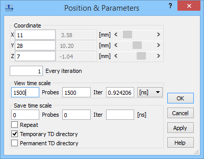
Fig. 2.7.1-3 Setting Envelope window parameters for tdr1.pro example.

We click over  button in Run tab to start the simulation and after about 1200 iterations we suspend it using  button. We obtain the results of simulation as presented in Fig. 2.7.1-4 and Fig. 2.7.1-5. Let us look at the first of them. Initially the signal is close to 0. Then when the pulse slope reaches the field testing point, it rises to the incident wave level. The incident wave level is maintained until the wave reflected from the end of the wide line reaches back the field testing point. The narrow line is inductive and thus the reflection coefficient is initially positive (causing that the E-field is amplified). However, since the narrow line is finally short-circuited, the steady state solution must bring reflection coefficient to the value of R=-1 and the field value to 0. The function TDR allows to read the reflection coefficient at any point in time. The reflection coefficient is presented as R=... in linear and dB scale after we place the first (blue) cursor at the point of measurement and the second (red) cursor at the level of the incident wave. This is exemplified in Fig. 2.7.1-4 where reading a late time reflection coefficient indicates a value very close to –1.

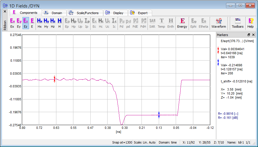
Fig.UG 2.7.1-4 E_z field versus time obtained in tdr1.pro example.

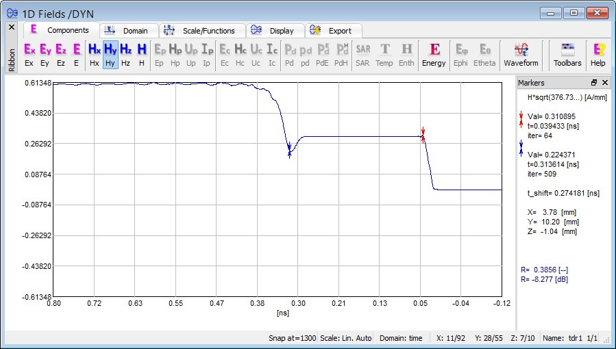
Fig. 2.7.1-5 H_y field versus time obtained in tdr1.pro example.

Fig. 2.7.1-5 presents the dual behaviour of the magnetic field variations. Moreover, in this case we would like to illustrate the possibility of measuring the distance between the field testing point and the discontinuity. We set the cursors at the beginning of the first pulse rise and the time point when the wave reflected from the discontinuity starts to perturb the waveform. We read that the time difference between these two points is 0.274 ns. After multiplying this value by the speed of the wave in teflon we obtain 57.68 mm. The distance to the discontinuity should be equal to half of that, i.e., 28.84 mm. In fact, we know that that distance is 32-3.36=28.64 mm. Thus in our virtual TDR experiment we are able to locate both the position of the discontinuity and its character (short circuited inductance).

Note that we have been using a step pulse of a limited spectrum (and thus finite rise-time). Let us now check what happens when we apply an abrupt step pulse. Let us return to QW-Editor and set in Edit Transmission Line Port: Step pulse. In fact, this step can be considered as the one with rise time equal to one FDTD iteration. In QW-Simulator we can read in Simulation Info tab of Simulator Log window that dt=0.00061614 ns for tdr1.pro analysis. Now run the simulation with such a step pulse. The results are presented in Fig. 2.7.1-6. They are essentially very similar to those of Fig. 2.7.1-4. However they are distorted by very high frequency components (with frequencies of the order of hundreds of GHz), which are not correctly treated by the FDTD method with 0.4 mm cell size set in tdr1.pro.

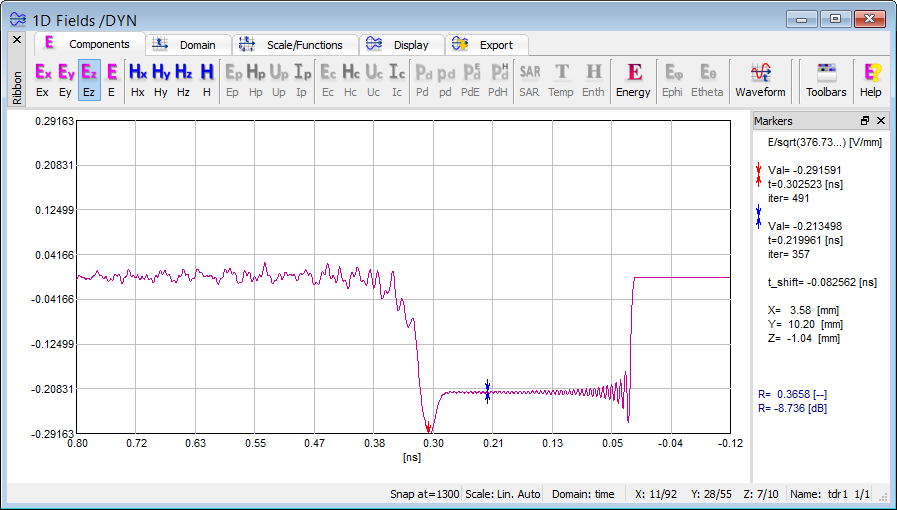
Fig. 2.7.1-6 E_z field versus time obtained in tdr1.pro example with an abrupt step pulse.