2.6 Dispersive media analysis
In this Section we consider dispersive media application in QW-V2D. We shall also present possibilities of performing arithmetical operations on the characteristics through the Config dialogue.
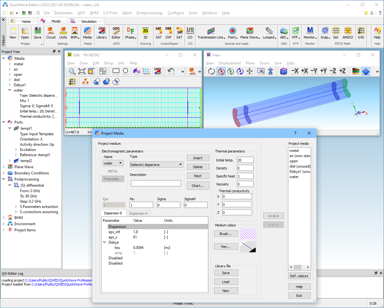
The Materials/Dispersive/water_v2d.pro example of Fig. 2.6-1 concerns a section of coaxial line filled with water. The Project Media dialogue visible in Fig. 2.6-1 shows that medium water is Dielectric dispersive, characterised with Debye model producing the following frequency-dependent complex permittivity:
er(w) = eps_inf + (eps_s - eps_inf) / (1 + j w tau)
Its parameters eps_inf (relative permittivity at infinite frequency),eps_s (static relative permittivity) and tau (relaxation time) are set after the book by K.S.Kunz, R.J.Luebbers, “Finite Difference Time Domain Method for Electromagnetics”, 1993 by CRC Press, Inc., Chapter 8.2.
Fig. 2.6-1 QW-Editor display of water_v2d.pro example with open Project Media dialogue.
Note that this project is defined in micrometers (see Units dialogue). Coaxial line radii are 75 mm/300 mm, and the applied discretisation (in Mesh Parameters dialogue) is 37.5 mm. Assuming a minimum of 10 cells per wavelength, this mesh allows covering the spectrum up to 800 GHz in air. Maximum permittivity of water is 81 and therefore this project has been set for the frequency range up to 80 GHz. As we will see, this has been a rather conservative choice: water permittivity decreases with increasing frequency, down to 20.90 at 30 GHz and 5.11 at 80 GHz. The coaxial line is excited by TEM mode and terminated with an absorbing port with effective permittivity equal to eps_inf.
We start the simulation with Start button. We may wish to verify if the dispersive medium has been correctly exported into QW-Simulator. After invoking Dispersive Media Info dialogue (Fig. 2.6-2) we choose Chart option, which reveal the dependence of the real and imaginary part of relative permittivity versus frequency as shown in Fig. 2.6-3.
Invoke the Results window to see the reflection and transmission characteristics versus frequency, as shown in Fig. 2.6-4. Note that reflections are very low (-140 dB) wide-band, even though the output port is well matched at high frequencies only, due to the eps_inf setting for effective permittivity. In fact, reflections from the output are compensated by the differential method of S-parameter extraction, due to the circuit being declared as reciprocal N-port in the S-Parameters dialogue of QW-Editor. Transmission drops from 0 dB at DC to -106 dB at 80 GHz, due to the increasing attenuation constant.
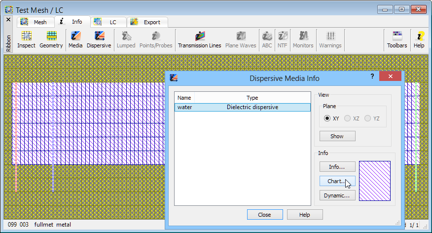
Fig. 2.6-2 QW-Simulator display of Dispersive Media Info dialogue.
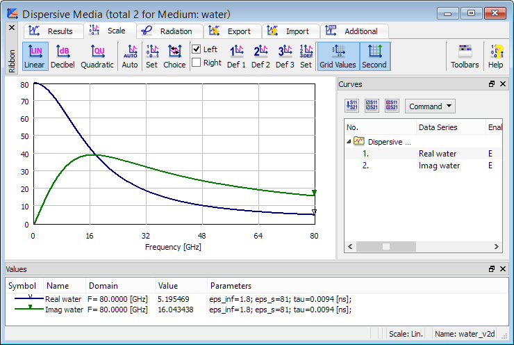
Fig. 2.6-3 QW-Simulator display of dispersive characteristic of water Materials/Dispersive/water_v2d.pro example.
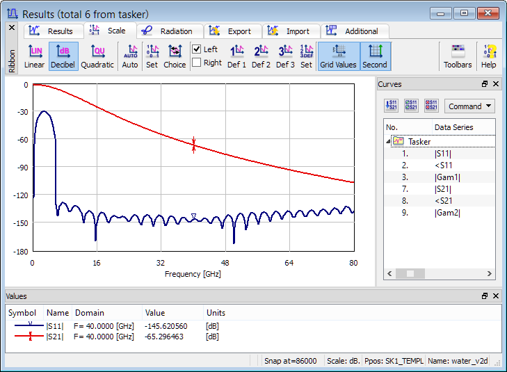
Fig. 2.6-4 QW-Simulator display of reflection and transmission characteristics in water_v2d.pro example.
Consider now the complex propagation constant and invoke once again the Results window with S-parameters results but in the extended S Results mode (![]() button). The extended mode is indicated by /EXT in the status bar, see Fig. 2.6-5. From |Gam1| and <Gam1 in the picture of Fig. 2.6-5, we can extract real and imaginary parts of complex permittivity as in the picture Fig. 2.6-6. To simplify this extraction, we have used |Gam1|calculated for the air-filled line of air_v2d.pro example available in the same directory. Note that full S-parameter data is saved with Save option; to save a single curve, we open Config dialogue highlight this curve and press. The absolute value of the phase constant in air has been saved in gamma0.da3 file.
button). The extended mode is indicated by /EXT in the status bar, see Fig. 2.6-5. From |Gam1| and <Gam1 in the picture of Fig. 2.6-5, we can extract real and imaginary parts of complex permittivity as in the picture Fig. 2.6-6. To simplify this extraction, we have used |Gam1|calculated for the air-filled line of air_v2d.pro example available in the same directory. Note that full S-parameter data is saved with Save option; to save a single curve, we open Config dialogue highlight this curve and press. The absolute value of the phase constant in air has been saved in gamma0.da3 file.
We open another Results window and load the reference curve with Load option. Denoting by γ the complex propagation in the water-filled line (Gam1) and by β0 the phase constant of the air-filled line (from gamma0.da3), we can calculate:
(γ / β0)2 = -ε’ + jε”
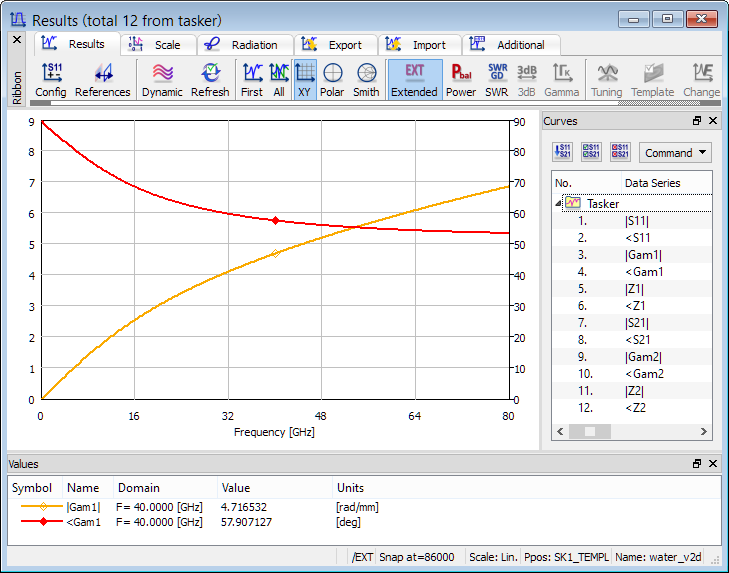
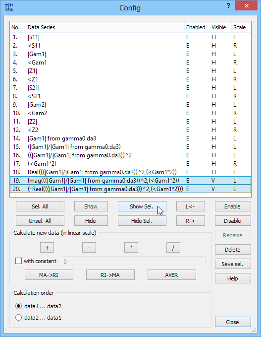
Fig. 2.6-5 QW-Simulator display of propagation constant in water_v2d.pro example and Config dialogue during mathematical operations.
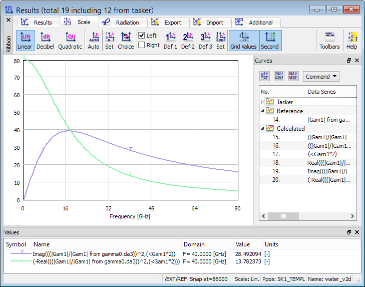
Fig. 2.6-6 QW-Simulator display of real and imaginary parts of relative complex permittivity extracted therefrom and Config dialogue during operations on two curves are shown.
We then open Config dialogue and perform the following sequence of operations:
- select curves No.3, 14 and press ![]() (see lower dialogue in Fig. 2.6-5),
(see lower dialogue in Fig. 2.6-5),
- select the new curve No.15 and press ![]() ,
,
- select curve No.4, check with constant box, insert 2 into the text field, press ![]() (see lower dialogue in Fig. 2.6-5),
(see lower dialogue in Fig. 2.6-5),
- select curves No.16, 17, press ![]() ,
,
- select the new curve No.18, press ![]() ,
,
- select curves No.19, 20, press ![]() .
.
The chart as in Fig. 2.6-6 appears. The green -Real(..) curve is ε’ and the violet curve Imag(..) is ε” for water. Colours and styles of the curves can be modified by highlighting the curve description in the legend, pressing right mouse button and invoking Edit Line dialogue. Scale can be set with Scaling dialogue.
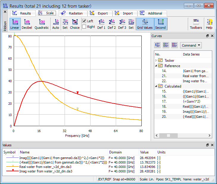
Fig. 2.6-7 Comparison of real and imaginary parts of relative complex permittivity in water_v2d.pro example obtained from |Gam1| and <Gam1 curves and from Dispersive Media Chart.