A dipole near electric wall
The present example considers a single dipole near electric wall.
A dipole near electric wall.
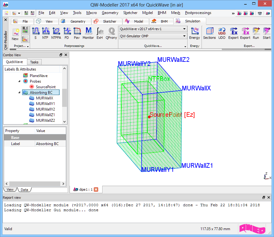
A dipole near electric wall project in QW-Modeller.
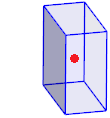
In this project, a single dipole is placed in a free space, near an electric symmetry plane (perpendicular to X axis). This scenario is equivalent to the one with two dipoles in a free space excited out-of-phase.
The dipole is placed in a volume of free space with the following side dimensions: 24 mm, 48 mm, and 48 mm in X, Y, and Z direction respectively. The electric symmetry plane is placed at x= 24 mm and the dipole is separated from it by a distance of 12 mm.
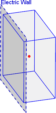
For the purpose of calculating radiation pattern, the NTF Box (green box), which is a virtual box determining the boundaries at which the near-to-far field transformation will be executed, is inserted in the project. The lower NTF Box wall along X axis coincides with the symmetry plane.
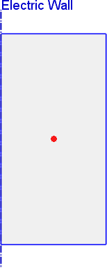
The exterior boundaries of the considered volume are absorbing except for the one where the symmetry plane is placed. The absorbing boundary conditions model the free space surrounding. In this case we use MUR absorbing boundary conditions in a form of MUR Box (blue box).
The radiation pattern calculations are set at 6.25 GHz and 12.5 GHz.
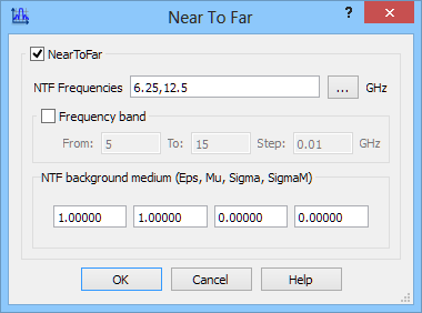
Near To Far postprocessing configuration dialogue.
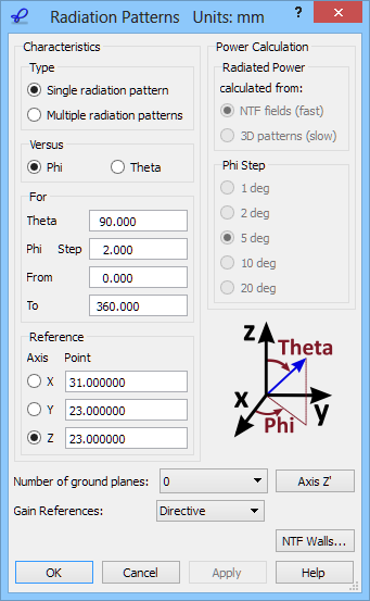
We wish to calculate the 2D radiation patterns versus angle Phi varying between 0 and 360 degrees with a step of 2 degrees. They will be calculated with a constant Theta angle equal to 90 degrees. The definition of the angles is explained in the lower right part of the 2D Radiation Patterns configuration dialogue. Note that this definition depends on the choice of the reference axis. The angle Theta is always counted from the reference axis (Z in the considered example). The angle Phi is always counted around it.
2D Radiation Patterns configuration dialogue.
The reference axis can be set to X, Y or Z by clicking respective radio buttons in the Axis column of the dialogue. There is also an option to define an arbitrary reference axis. For an example of application of this option, please refer to the Two dipoles in free space excited in phase.
We can also set the reference point or in other words the origin of the coordinate system for the NTF transformation. The position of the reference point does not influence the absolute values of the radiation patterns (in lossless NTF background medium) but it does influence their phase characteristics. Moving the reference point can be helpful in a search for the antenna electrical centre. The reference point position is expressed in the same coordinates and units as those used in the project and defined in the user input interface. To recall what units have been used, we can just take a look at the title bar of the window. In the considered example we see Units: mm.
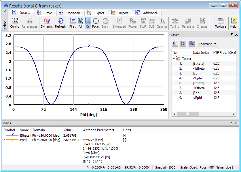
2D radiation patterns calculated at 6.25 GHz.
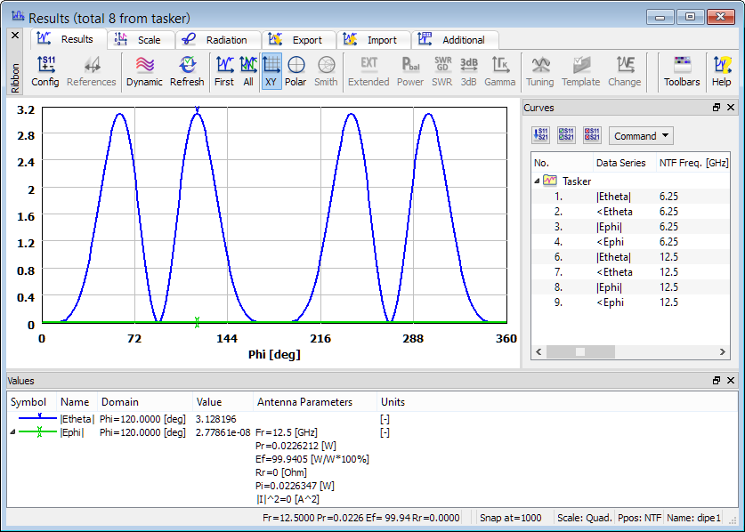
2D radiation patterns calculated at 12.5 GHz.
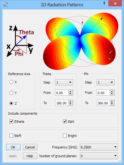
3D radiation pattern, with both Phi and Theta varying in steps, can be calculated in the 3D Radiation Pattern window. The 3D Radiation Patterns dialogue allows setting the reference axis and steps for angles Phi and Theta, defined with respect to that axis in the same way as for the 2D radiation pattern case. A single calculation frequency is also selected.
3D Radiation Patterns configuration dialogue.
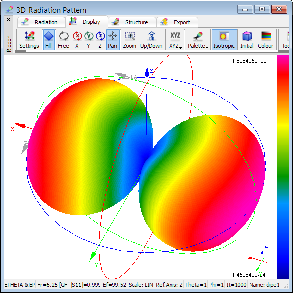
3D radiation pattern calculated at 6.25 GHz.
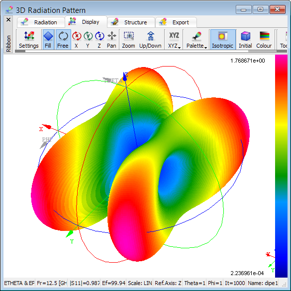
3D radiation pattern calculated at 12.5 GHz.