
6.1.3 Dissipated power and dissipated power density
QW-3D allows simulation of circuits with electric volumetric losses described by conductivity s [S/m] and with magnetic volumetric losses described by magnetic conductivity sm [W/m]. It can also apply a surface loss model in the case of metals characterised by large but finite conductivity s [S/m].
The influence of losses on circuit performance is quantitatively described by such results of the analysis as: radiation efficiency of antennas, Q-factors of resonators and power dissipated in the lossy objects, or power balance in S-parameters extraction. For qualitative purposes, calculations and time domain distribution displays of:
dissipated power per cell (Pd)
dissipated power density (pd)
dissipated electric power per cell (PdE) – power dissipated due to losses in electric field
dissipated magnetic power per cell (PdH) – power dissipated due to losses in magnetic field
in the circuit have also been enabled.
The calculations of the dissipated powers are somewhat different in QW-V2D than in QW-3D, due to its specificity:
dissipated power per ring (Pd)
dissipated power density (pd)
dissipated electric power per ring (PdE) – power dissipated due to losses in electric field
dissipated magnetic power per ring (PdH) – power dissipated due to losses in magnetic field
The meaning of ring in QW-V2D is as follows:
ring=2*π*r*dx*dy
where dx, dy stand for the cell size in X and Y direction, respectively, and r is the radius of the ring associated with a middle of the cell along Y axis.
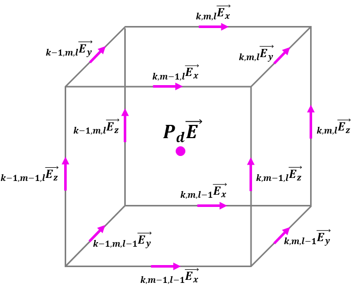
At this point it is necessary to give the user an information concerning the procedure of calculating the power dissipated. Note that the power dissipated in a cell is calculated from the electric and magnetic field components staggered in space by averaging. Software calculates dissipated electric power (PdE) from the electric field components as shown in Field components included in calculation of electric dissipated power picture, where k,m,l stand for cell indexes. The dissipated magnetic power (PdH) is calculated from the magnetic field components shown in Field components included in calculation of magnetic dissipated power picture (k,m,l stand for cell indexes). The total dissipated power is calculated as a sum of dissipated electric power and dissipated magnetic power (from the field components as shown in Field components included in calculation of total dissipated power picture).
Field components included in calculation of electric dissipated power in the presented cell, centred at the cell centre marked by the magenta dot.
PdE= f (k,m,l Ex, k,m-1,l Ex, k-1,m,l Ey, k,m,l Ey, k,m,l-1 Ex, k,m-1,l-1 Ex, k-1,m,l-1 Ey, k,m,l-1 Ey, k-1,m-1,l Ez, k,m‑1,l Ez, k-1m,l Ez, k,m,l Ez)
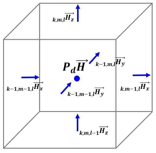
Field components included in calculation of magnetic dissipated power in the presented cell, centred at the cell centre marked by blue dot.
PdH= f (k-1,m-1,l Hx, k,m-1,l Hx, k-1,m-1,l Hy, k-1m,l Hy, k,m,l-1 Hz, k,m,l Hz)
Field components included in calculation of total dissipated power Pd in the presented cell, centred at the cell centre marked by black dot.
Pd= PdE + PdH
The above figures show that power dissipated in each FDTD cell is averaged from several field components - but also each field component contributes to dissipated power and energy in more than one cell. The FDTD algorithm naturally produces dissipated power and energy associated with a particular field component and its surrounding volume. In QW-Simulator, the power is subsequently distributed among cells sharing these field components proportionally to relative dimensions of such cell, and their relative conductivities. Power portions assigned to metal cells (PEC or metallic) are zero.
The time domain displays showing the distribution of the dissipated power (total, electric, and magnetic) and dissipated power density is available in a form of:
· 1D distribution display
· 2D distribution display
· 3D distribution display
In case of 1D distribution displays, QuickWave allows monitoring the dissipated power (total, electric, magnetic) and dissipated power density along any line parallel to one of coordinate axes or in a particular point of the circuit versus time. The 1D monitoring delivers instantaneous and envelope (time-maxima) values of the chosen quantity and is available in 1D Fields window. General discussion concerning the 1D distribution monitoring is given in Monitoring along specified line and versus time.
In the second option QW-3D enables monitoring the time-dependent 2D distribution of the dissipated power (total, electric, magnetic) and dissipated power density in the circuit, available for every FDTD layer along each of three axes. The distributions of the above quantities are available in 2D/3D Fields Distribution window, which offers several different options for adjusting the distribution display to the user’s needs (e.g. display type, scales, etc.).
Dissipated power is calculated in [W]. Dissipated power density equals to dissipated power divided by the volume of cell (shown in Field components included in calculation of total dissipated power picture), thus its unit is [W/mm3]. It is worth noting that their numerical value within each FDTD cell can be read in Thermal mode of display.
Attention: Within a homogeneous isotropic medium, density of power dissipated in the electric field is equal the product of total electric field and conductivity. Note that E total is differently averaged in space than the electric field components contributing to dissipated power anddissipated power density (compare Field components included in calculation of total E-field and Field components included in calculation of electric dissipated power pictures). Hence the numerically calculated value of power dissipated density may differ from the product of E total and medium conductivity in the cell. This discrepancy is a measure of the influence of field components averaging over the cell on the accuracy of power and total field extraction. Note that H total is averaged in space in the same way as the magnetic field components contributing to power dissipated and power dissipated density (compare Field components included in calculation of total H-field and Field components included in calculation of magnetic dissipated power pictures).
The 2D distribution display in 2D/3D Fields Distribution window allows primarily monitoring the instantaneous values of dissipated power. Time-maximum of power dissipated in each cell can be found by switching to Envelope Max option. In many applications, such as microwave heating, average power dissipated in a sinusoidally-excited circuit is of interest to the user. Note that in a general case the relation between average power Pav and maximum power Pmax is not straightforward; all we know is that:
Pav = 0.5..1.0 Pmax
To obviate the above ambiguity, rigorous calculations of average dissipated power have been implemented in QW-3D. The average power is defined as:
Pav = 0.5 (Pmin + Pmax)
where Pmin is time-minimum of dissipated power.
The distribution of average dissipated power can be enabled with Envelope Avr option.
The distribution of dissipated power and dissipated power density is physically meaningful in the steady-state sinusoidal excitation regime. However sometimes we are interested in the distribution of the total power dissipated when the circuit is excited by a pulse of limited duration. This will be a distribution of the time integral of dissipated power (dissipated power density), thus the distribution of the total energy converted into heat during the simulated process. The distribution of the time integral of dissipated power (òPd), dissipated power density (òpd), dissipated electric power (òPdE), and dissipated magnetic power (òPdH) are available in the 2D/3D Fields tab or 2D/3D Fields Distribution window. Invoking this option starts the time integration of the chosen quantity in each FDTD cell at each time-step. Two remarks must be made at this point:
- To get valuable distribution display, the time integration of dissipated power (dissipated power density) must start from the first FDTD iteration.
- Invoking time integration of the dissipated power (dissipated power density) enables calculation of the dissipated power at every time-step in each FDTD cell, making the entire process resources consuming (the user may notice the decrease of simulation speed given in FDTD iterations per second).
The time-dependent dissipated power and dissipated power density distribution can be also viewed as 3D displays. This feature is enabled in the 2D/3D Fields Distribution window and allows watching the instantaneous, time-maximum, and time-average values of dissipated power and dissipated power density.