
2.13.1 A parallel-plate transmission line
In previous Sections we have demonstrated various options for visualising field patterns in a plane or along a straight line. In many practical cases, however, we may prefer to observe not only the spatial patterns, but also integral quantities, such as a line integral of the electric field along a pre-defined integration path. If the field is potential, then this integral has the physical meaning of voltage. Knowing the voltage between two metal objects allows predicting the hazards of arcing and electric breakdown.
The path of integration may be defined by the user with UDO objects from the contours library. Three of the available UDOs allow setting the path composed of 1, 3 or 7 segments (spanned between 2, 4 or 8 points, respectively). Another UDO facilitates reading the number of points and their coordinates from a text file. The points may be arbitrarily located in space but they will be snapped to the nearest mesh point (cell vertex), similarly as in the case of point sources. Each segment will be decomposed into a Manhattan-style route along cell edges. During the simulation, the electric field is integrated along the path, and this integral will be Fourier-transformed by FD-Probing post-processing, analogously as voltages at lumped sources and probes.
A group of examples in Various/Contours directory demonstrates the usage of contourE.udo objects. For benchmarking purposes, the contours are defined inside a parallel-plate TEM line, where the results of integration can be analytically predicted.
Fig. 2.13.1-1 The view of contour2.pro in QW-Editor.
Let us start with ..\Various\Contours\contour2.pro example. Fig. 2.13.1-1 shows the considered structure. The parallel-plate transmission line is located along the x-axis and supports a TEM wave with Ez and Hy field components. It has been defined via the elib/recwg/pp.udo library object. The path of integration is marked in magenta. It has been defined via the elib/contours/contourE4.udo, between two terminal points requested at (50,0,0) and (50,0,10) and effectively snapped to (50,0.5,0) and (50,0.5,10). Hence the integrated field will have the significance of voltage between the two metal plates.
The I/O Ports Parameters dialogue shows that a delta pulse will be applied to excite the TEM wave. The Processing/Postprocessing dialogue shows that two types of post-processing will be conducted: S-Parameters (between the two ports) and FD-Probing (of integrated voltage), both between 0 and 30 GHz. In typical applications of the software setting of the delta pulse is not recommended since it may excite out-of-band resonances that slow down simulation convergence. In this example, the circuit is non-resonant and matched. The delta pulse will excite a wave with (theoretically) frequency-independent available power. With source amplitude set to unity the time-maximum available power is 1W. Since the cross-section of the parallel-plate line is square and the line is filled with air, its characteristic impedance is equal to free-space impedance and voltage amplitude should be (120 p) -0.5. Considering that all voltages and electric fields in QW-Simulator are normalised by (120 p) -0.5 (see Electromagnetic fields), we expect FD-Probing to show the normalised voltage of unity.
Let us start the simulation by pressing ![]() button in the Simulation tab of QW-Editor. The Simulator Log confirms that the numerically extracted transmission line impedance is approximately equal to the free-space impedance:
button in the Simulation tab of QW-Editor. The Simulator Log confirms that the numerically extracted transmission line impedance is approximately equal to the free-space impedance:
Fig. 2.13.1-2 Reflection, transmission and characteristic impedance in extracted by S-Parameters post-processing in extended mode of QW-Simulator, with manually set left and right scales.
Pressing ![]() button in Results tab of QW-Simulator invokes Results window with S-Parameters results in extended mode as shown in Fig. 2.13.1-2. Non-dispersive transmission line impedance and good matching is confirmed over the considered frequency range. Pressing
button in Results tab of QW-Simulator invokes Results window with S-Parameters results in extended mode as shown in Fig. 2.13.1-2. Non-dispersive transmission line impedance and good matching is confirmed over the considered frequency range. Pressing ![]() button in Results tab of QW-Simulator invokes Results window with voltage amplitude as in Fig. 2.13.1-3. At low frequencies it precisely equals unity and then slowly increases. This is due to the way that template sources are numerically applied in the software. An explicit excitation method is used which causes frequency-variation of source output impedance and a resulting slow increase in the source numerically available power with frequency. As a rule-of-thumb, field amplitudes increase by 4% at 10 cells per wavelength. The integrated value of voltage follows this effect.
button in Results tab of QW-Simulator invokes Results window with voltage amplitude as in Fig. 2.13.1-3. At low frequencies it precisely equals unity and then slowly increases. This is due to the way that template sources are numerically applied in the software. An explicit excitation method is used which causes frequency-variation of source output impedance and a resulting slow increase in the source numerically available power with frequency. As a rule-of-thumb, field amplitudes increase by 4% at 10 cells per wavelength. The integrated value of voltage follows this effect.
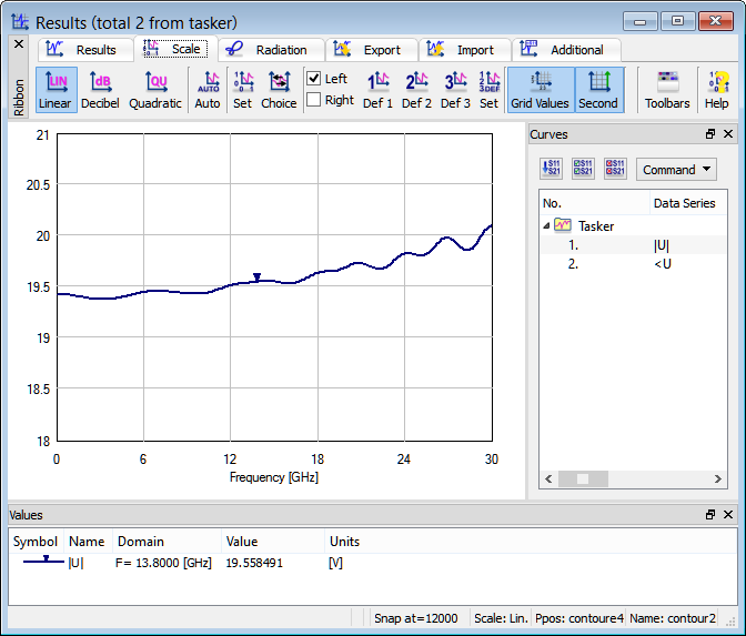
Fig. 2.13.1-3 Voltage amplitude extracted by FD-Probing in contour2 (and contour2a) example.
Let us now proceed to the ..\Various\Contours\contour2a.pro example. As shown in Fig. 2.13.1-4, the path of integration is now tilted with respect to the y-axis, but contained in the same xz-cross-section of the transmission line. Hence the integrated quantity should maintain the physical meaning of voltage. Indeed, upon pressing ![]() button from Results tab of QW-Simulator we obtain an identical display as in Fig. 2.13.1-3.
button from Results tab of QW-Simulator we obtain an identical display as in Fig. 2.13.1-3.
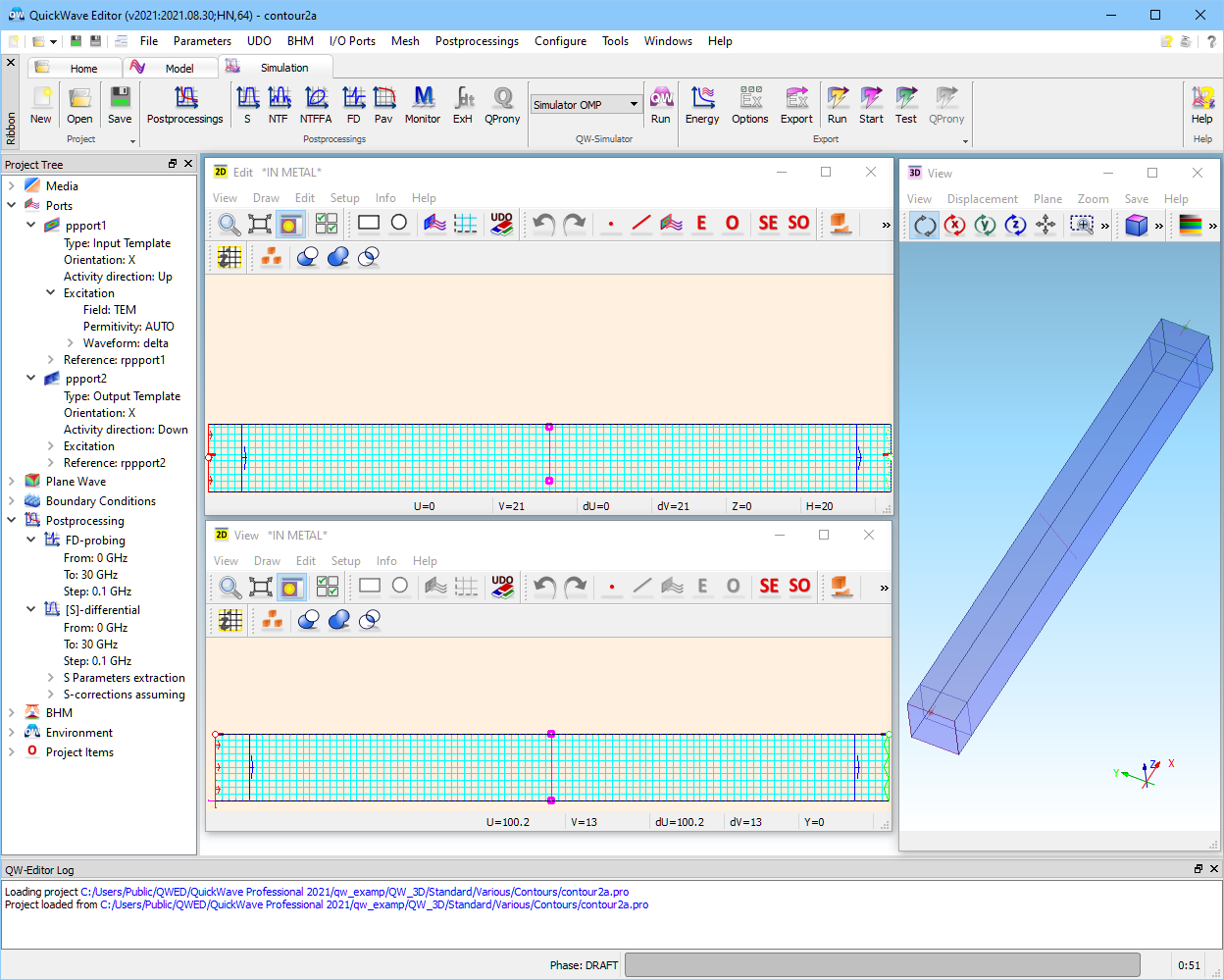
Fig. 2.13.1-4 The view of contour2a.pro in QW-Editor.
In ..\Various\Contours\contour2b.pro example the path of integration is inclined with respect to the x-direction and spans the distance of 20 mm along the transmission line. The structure is shown in Fig. 2.13.1‑5 and the results of FD-Probing post-processing in Fig. 2.13.1-6. At DC wavelength is infinite, there is no field variation along the line, and the integrated quantity retains the significance of voltage and unity absolute value. Above DC, it becomes voltage multiplied by the integral of cos(βxx) function with respect to the x-variable. Therefore the characteristic of Fig. 2.13.1-6 has zeros at frequencies where wavelength is a sub-multiple of 20 mm (slightly shifted towards lower frequencies due to numerical dispersion of the FDTD method - by approximately 1% at 10 cells per wavelength). Its maxima occur where 20 mm accommodates an odd number of half-wavelength, and follow the f -1 envelope.
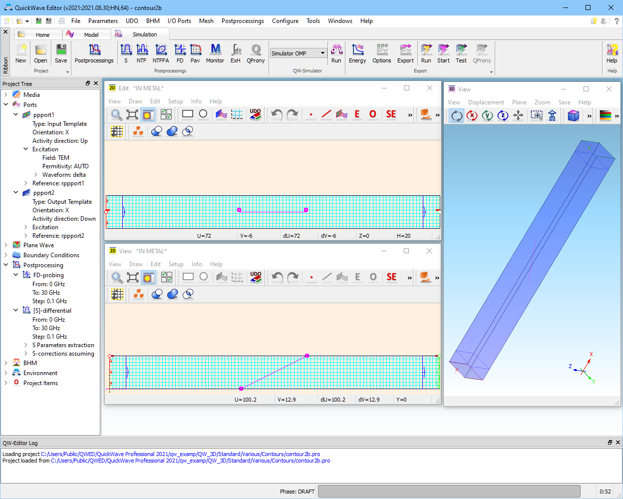
Fig. 2.13.1-5 The view of contour2b.pro in QW-Editor.
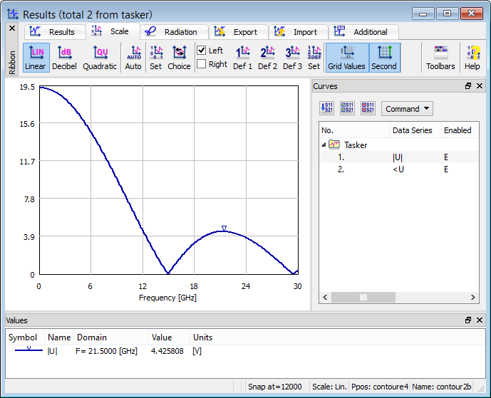
Fig. 2.13.1-6 Voltage amplitude extracted by FD-Probing in contour2b example.
Finally, in contour2c.pro example we take advantage of the fact that contourE4.udo applied in the project definition allows setting four path points. Their location shown in Fig. 2.13.1-7 is (40,0,0), (40,0,5), (60,0,5), (60,0,10) and entails that the Ez field will be integrated along two equal-length segments, separated by a electric distance varying with frequency. The results of Fig. 2.13.1-8 correctly show zeros where the distance is an odd-multiple of half-wavelength and maxima where it is a multiple of wavelength. The values of maxima gradually increase by up to 4% at 10 cells per wavelength, as explained with reference to Fig. 2.13.1-3.

Fig. 2.13.1-7 The view of contour2c.pro in QW-Editor.
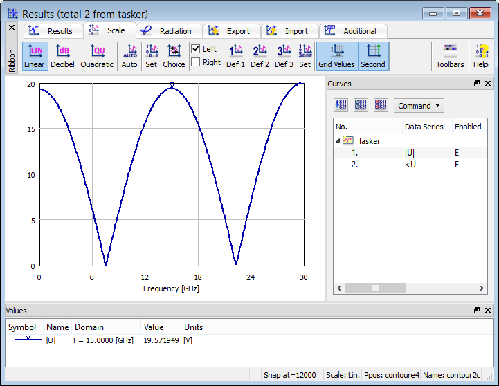
Fig. 2.13.1-8 Voltage amplitude extracted by FD-Probing in contour2c example.

