
2.2.2 Advanced S-parameter problems for waveguide-to-coax example
S-parameters below the cutoff frequency
Let us now repeat the analysis of wgtocx1.pro with modified dimensions (“coax.pos.x (OX)=25” and “antenna length (E)=2.2”). But this time we will use a wider frequency band from 10 to 30 GHz. Those settings were made in the project wgtocx2.pro. With a wider frequency band we excite the circuit at a higher resonant frequency (about 27 GHz) and also below the waveguide cutoff. Both excite slowly decaying processes and make the convergence to the final characteristics slower. Thus we run the simulation up to about 6000 iterations before suspending it. Then we open a Results window and display the following curves:|S11|, |S21|, |Gam1| and |Gam2|. The display is presented in Fig. 2.2.2-1.
Fig. 2.2.2-1 Results of simulation of wgtocx2.pro in a wider frequency band.
|Gam1| and |Gam2| denote the absolute values of propagation constants in the transmission lines terminated by ports 1 and 2, respectively. It can be seen that at port 1 (waveguide input) the propagation constant drops to 0 at the waveguide cutoff (15 GHz), while at the TEM output |Gam2| is naturally proportional to the frequency.
Let us have a closer look at the values of |S11| and |S21| below the cutoff frequency. Naturally |S21| drops fast with decrease of the frequency. But what may seem less intuitive, there is also a fast decrease of |S11|. This is because even below the cutoff a long section of waveguide is reflectionless and thus its |S11| must tend to zero with the length of the section increasing. Let us also note that zero reflection does not imply any transmission of a real power into the guide since the characteristic impedance of the guide (equal to the reference impedance for S-parameter definition) is imaginary below the cutoff frequency. The list of all parameters that can be calculated below cutoff frequency is given in Below cutoff calculations. More discussion about interpretation of the S-Parameters below cutoff can be found in ref. [44].
Extended S-parameters
Let us take a look at the list of the available characteristics listed in the Config dialogue (Fig. 2.2.2-2). We have 6 items, which provide complete information for most applications. However, in some specific applications the user may require additional information about the phase angle of the propagation constant and about the changes in the characteristic impedances of the port lines (which are also reference impedances for the calculated S-matrix). To extract this extended information we need to activate Extended Results option for Results window e.g. by pressing Extended button. The list is extended to 12 items as seen in Fig. 2.2.2-2.
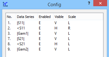

Fig. 2.2.2-2 List of available characteristics with standard and extended results options.
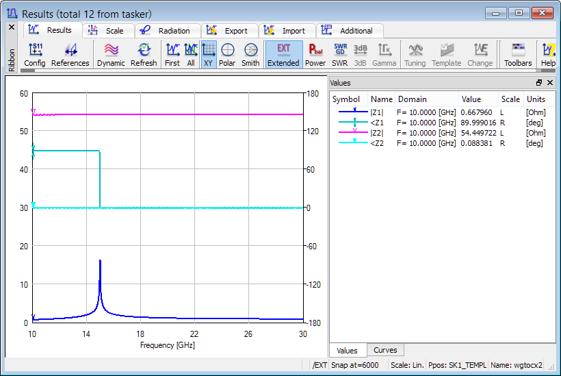
Fig. 2.2.2-3 Display of characteristic input/output impedances available in extended results options.
Let us have a look at the characteristic impedances as displayed in Fig. 2.2.2-3. At the TEM output we have a constant and real impedance in the entire frequency band. At the waveguide input the impedance is real (<Z1=0) above the cutoff and imaginary (<Z1=90o) below the cutoff. The absolute value of the impedance changes in a way typical to a hollow waveguide TE mode that is, it rises when approaching the cutoff frequency. It is well known that a characteristic impedance of a waveguide is not uniquely definable and it is a subject of arbitrary normalisation (see ref. [44]). In QW-3D we normalize the characteristic impedance of a waveguide mode in such a way that it is equal to unity at the frequency at which the mode template has been calculated. In the considered example the input mode template has been calculated at 22.5 GHz and that is why |Z1|=1 at that frequency. Note however that in the case of TEM line for which the unique definition of impedance is possible, QW-3D indicates the actual impedance being Z2=54.4 W in our case.
It has been mentioned in the previous Section that the S-Parameters are extracted with respect to reference planes situated at some distance from the ports and that we can virtually move the reference plane during results calculation. Let us return to the results of analysis already considered in Fig. 2.2.2-1. We save them on disk. Then we invoke Reference Location dialogue (using References option of Results window) as presented in Fig. 2.2.2-4. Let us now try to move the virtual reference planes of both ports to the position of the coaxial line antenna inserted into the waveguide. Thus we set in Port 1 New location =25 and in Port 2 New Location = 3. To compare the transformed results with the original ones we read the saved results from disk using Load option in Import tab. After accessing the Config dialogue list we choose for display: |S21| and <S21 for both the current and original (read from disk) results. Comparison of them is shown in Fig. 2.2.2-5. As expected, moving the reference plane makes the phase characteristics more flat (green line versus red line) and does not change|S21|above the waveguide cutoff (where the blue line is hidden under the yellow line). It is interesting to note that the software takes into account the real part of the propagation constant below the cutoff and appropriately corrects |S21| for low frequencies. That is why for example for 12 GHz |S21| rises from 0.0179 to 0.697.
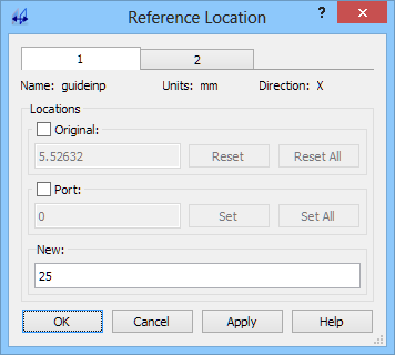
Fig. 2.2.2-4 Reference Location dialogue for changing virtual location of the reference planes of ports.

Fig. 2.2.2-5 Results of calculations of the considered example with the original reference planes (orange + red) and the reference planes virtually moved to the position of the coax antenna (blue + green).
Disscussion regarding the feature enabling virtual shift of the reference plane is given in S-Parameters.
Power balance
Sometimes we are interested in the power balance of the analysed structure. In other words, we would like to know what part of the power injected into the circuit is dissipated in all defined ports. Consider the results like those shown in Fig. 2.2.2-1. To calculate the power balance characteristic, activate Power option in Results windows or open two additional Results windows by pressing Power Balance button in the Results tab of QW-Simulator. Now we can see that the list of available curves offers either Pow.SK1 or Pow.Bal. to be displayed, with Extended Results off and on, respectively.
Pow.SK1 has a slightly different meaning than Pow.Bal. With the standard S-Parameters we do not extract the information about the phase of the reference impedance at each port. In such a case the power balance is calculated as:
Pow.SK1 = sqrt(|S11|2 +|S21|2).
In the case of imaginary or complex reference impedances (like for example in waveguides below the cutoff frequency) this formula does not describe the actual balance of input and output power.
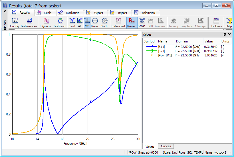
Fig. 2.2.2-6a Results of simulation of wgtocx2.pro including the power balance characteristic with standard (non-extended) S-parameters.
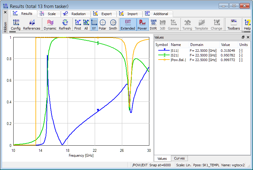
Fig. 2.2.2-6b Results of simulation of wgtocx2.pro including the power balance characteristic with extended S-parameters.
In the case of extended S-parameters the software calculates the actual power passing through each of the ports (contained in the mode assigned to a particular port). In such a case the power balance shows a square root of the ratio of the power dissipated in the load (or loads, in the case of multiports) to the power actually injected into the circuit from Port 1 working as the input. When Port 1 is unmatched or works below cut-off, the injected power may drop to zero. To avoid ill-conditioned calculations, Pow.Bal is set to zero when the injected power drops below 0.001 W threshold. It is recommended to refer to Power Balance for more details on power balance calculation and interpretation.
Displays of |S11|and |S21|together with Pow.SK1 in the case of using standard S-parameters are presented in Fig. 2.2.2-6a while the results obtained with extended S-parameters are shown in Fig. 2.2.2-6b. As expected, clear differences are visible below the waveguide cutoff frequency.
It is worth noting at this point that if the power balance does not converge to unity in a case of a lossless structure, this may indicate that some of the energy is dissipated in the source or/and load in modes not considered in the S-parameter extraction. Displays of Fig. 2.2.2-6a and Fig. 2.2.2-6b show a good example of such a case. We can see that at the frequency 27.2 GHz power balance drops to the value of about 0.5. The reason is that at this frequency much of the energy transmitted to the output is coupled to a waveguide mode in the coaxial line. This energy is ignored during calculation of |S21| since Port 2 has been defined at the TEM mode. To have full description of the circuit at that frequency we would need to define the structure as a three-port with the third port associated with the first waveguide mode in the output coax. This kind of multi-port approach will be considered in further examples.
Now, consider the difference in power balance display in the case of standard and extended S-parameters below the cutoff frequency of the waveguide. In the case of standard S-parameters (Fig. 2.2.2-6a) the power balance is not correctly calculated below 15 GHz. It can be seen that the power balance calculated with extended S-parameters (Fig. 2.2.2-6b) displays a value close to 1 even below 15 GHz, despite the fact that characteristic impedance of the input line is imaginary and that the real power injected into the circuits drops very fast with diminishing frequency. This confirms consistency of the S-parameter extraction even below the cutoff frequency of the waveguide. It can be seen in Fig. 2.2.2-6b that below 13.2 GHz the power balance shows 0. This indicates that the real power injected into the circuit at these frequencies is so small that the software cannot calculate the power balance with acceptable accuracy and sets the result to zero to avoid displaying a curve of irrelevant shape.
Note: The above-described option of calculating power balance with extended S-parameters is available only when the results are displayed during the simulation. The display of saved results stored on disk uses always the power balance formula for the standard S-parameters (sqrt(|S11|2 +|S21|2).
Excitation from one or more ports
You may have noted that so far we have been exciting the circuit at the input and calculating only two elements S11 and S21 of the four-element S-matrix. A question may arise: how to calculate a full S-matrix. To answer this question let us return to the S-Parameters dialogue of QW-Editor like the one presented in Fig. 2.2.2-7. Until now, we have been calculating S-parameters with an option Sk1 at reference planes. Sk1 means that we will use only one excitation from Port 1. At reference planes is compatible with the fact of using differential method of S-parameter extraction. The alternative is Smn at reference planes. In the latter case the software will calculate the entire S-matrix after consecutive excitations from Port 1 and Port 2. Such a way of calculating S-parameters is normally sequential, which means that the software will first calculate S11 and S21 after excitation from Port 1 and simulation over the declared number (5000 in Fig. 2.2.2-7) of FDTD iterations. Then it will excite the structure from Port 2 and calculate S12 and S22. At the end it will perform matrix operations to correct mutually the results obtained with excitation from each port, and display the final result. For more information concerning the two options of S-Parameters post-processing calculation, refer to S-Parameters.
Let us run the example with the above-discussed settings: Smn at reference planes, Sequential, which is wgtocx2smn.pro. After performing 10000 iterations (5000 with excitation from each port) the QW-Simulator stops. Assuming that we use standard (not extended) S-parameters but with Power balance we should obtain in the Config dialogue the list as shown in Fig. 2.2.2-8. We can see that we have 12 items including all S-matrix elements, two propagation constants and two power balances obtained with excitations from Port 1 and Port 2.
The results of calculation of S-matrix elements are presented in Fig. 2.2.2-9. It is visible that in the entire frequency band |S21|=|S12|, which is a direct consequence of the circuit reciprocity. Moreover, in the band between 15 GHz and 25 GHz we also have |S11| =|S22|. The latter relation is due to the fact that in this band the circuit is a lossless reciprocal two-port with real reference impedances. Above 25 GHz some of the energy is leaking into the waveguide mode in the coaxial like thus creating a kind of “losses” from the viewpoint of a two-port structure. Below 15 GHz the input reference impedance becomes imaginary and thus the relation |S11|=|S22|does not hold even for a lossless reciprocal two-port (as explained in the ref. [44]).
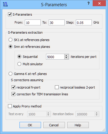
Fig. 2.2.2-7 S-Parameters dialogue of wgtocx2smn.pro.
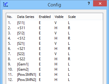
Fig. 2.2.2-8 List of parameters calculated with the option Smn at reference planes.

Fig. 2.2.2-9 Results of S-matrix calculations for wgtocx2smn.pro with the option Smn at reference planes.
So far we have been using the option Sequential putting aside Multisimulator possibility. In the Multisimulator case the software will create two simulators being objects within QW‑Simulator. Note that QW-Simulator has been developed in such a way that many simulator objects can exist and operate concurrently. In this case, one simulator will be running the FDTD analysis of wgtocx1 project with excitation applied from Port 1, and thus extracting S11and S21. The other simulator will be running the FDTD analysis of wgtocx1 project with excitation applied from Port 2, and thus extracting S22 and S12. The Smn postprocessing functions will be importing data from both simulators on-line, and also on-line performing mutual corrections. Therefore the intermediate results watched during the analysis will already be mutually corrected; this is an important advantage with respect to the sequential mode where only the final result is mutually corrected. The other advantage is that the number of iterations per port does not have to be predefined, and the decision about terminating the analysis is made dynamically by the user as in the case of single-port excitation. However, memory occupation increases by a factor of two, which is a disadvantage in the case of analysing large problems on low-memory computers. The computing time remains unchanged: although the total number of iterations is reduced by a factor of two, the number of operations per iteration is doubled.
For detailed discussion concerning all post-processing options available in S-Parameters dialogue refer to S-Parameters.