2.3.4      Wire antenna

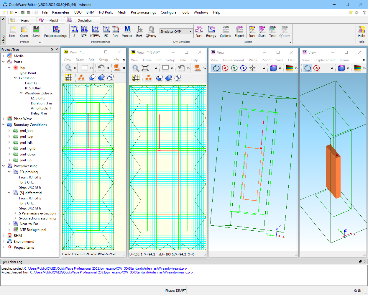
We will consider simulation of a simplified model of a mobile handset with a wire antenna, as presented in Fig. 2.3.4-1.The structure has been originally measured by Jensen and Rahmat-Samii and presented in “Performance analysis of antennas for hand-held transceivers using FD-TD”,IEEE Trans. Antennas Propag., vol. AP-42, No.8, Aug.1994, pp.1106-1113. It has been prepared for QW-3D simulation and stored in the file: ..|Antennas\Wireant\wireant.pro.

Fig. 2.3.4-1 A simplified handset model used in wireant.pro.

The project is composed of four objects called from standard QW-3D libraries. Press  to see the list of these objects (marked as UDO objects). They are:

body -  describing the body of the handset (generated by a call to ..\basic\solid.udo);

pmlntf -  describing the Near-to-Far box surrounded by Perfectly Matched Layer (PML) box (generated by a call to ..\boxes\pmlntf.udo);

inp -  describing the input lumped (point) source (generated by calls to ..\ports\ point.udo);

wire1 -  describing the antenna wire (generated by calls to ..\wires\ wire1.udo);

Here are some remarks concerning the projects:

§  Four mesh snapping planes (surrounding the body of the handset) have been generated using a procedure described in Planar circuit and supplemented to the above objects;

§  There is no need to add the mesh snapping planes for the wire since the software snaps the FDTD mesh to the wire anyway.

§  In the Processing/Postprocessing dialogue we can see that three different post-processings were defined: S-Parameters, Near To Far, and FD-Probing. The last one has been declared here because it provides additional information concerning the driving point impedance seen from the antenna excitation point. This information can be of direct interest in wire antenna design.

Fig. 2.3.4-2 shows calculated values of |S11| versus frequency, displayed in Results window ( button in S-Parameters section of Results tab in QW-Simulator). They are in agreement with the measurements data provided by Jensen and Rahmat Samii.

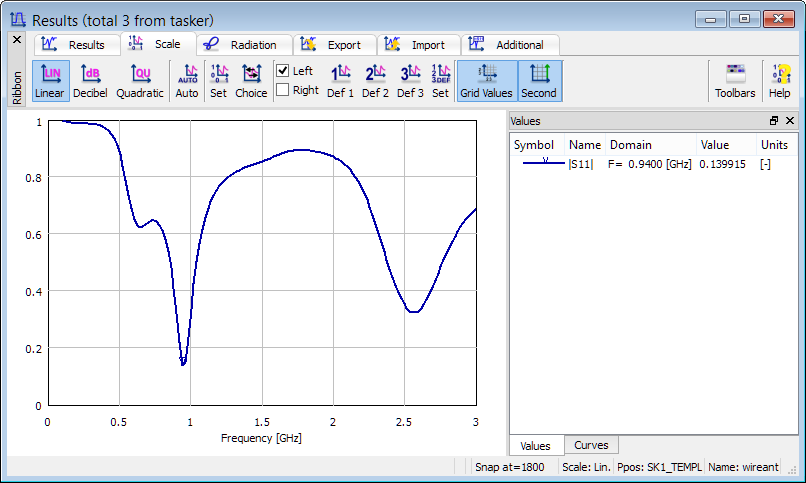
Fig. 2.3.4-2 The results of simulation of the return loss of wireant.pro.

Fig. 2.3.4-3 shows the Results window with 2D radiation pattern versus angle Theta for Phi=90° with reference axis Z, i.e., in zy-plane, obtained after pressing  button in 2D Radiation Pattern section of Results tab in QW-Simulator. Note that radiation is more intense down along z-axis (on the side of the body of the handset) than up along z-axis (on the side of antenna). Of the two upward beams, the stronger one in the negative y-direction since the antenna is offset from the handset centre in the negative y-direction.

Fig. 2.3.4-3 The results of simulation of the radiation pattern of wireant.pro.

NTF post-processing extracts total power radiated by the antenna Pr. Note that NTF frequency 0.940 GHz is also one of the frequency points in S-Parameters and FD-Probing post-processings, both of which are applied from 0.1 to 3 GHz, with step 0.02 GHz. Taking power delivered by the source to the antenna from S-Parameters calculation the software is able to calculate radiation efficiency Ef. It has practically reached 100%, which confirms convergence of the results for a lossless antenna. Similarly, taking current flowing between the source and the antenna from FD-Probing, the software calculates radiation resistance Rr. However, NTF frequency 0.915 GHz does not coincide with S-Parameters and FD-Probing post-processings frequency points, so Ef and Rr are not calculated.

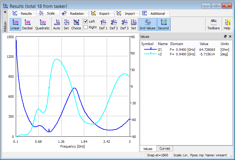
Fig. 2.3.4-4 The input impedance of the wire antenna of wireant.pro obtained using FD-Probing post-processing.

Fig. 2.3.4-4 shows the results for driving point impedance seen from the source and obtained with FD-Probing post-processing. Use  button from Results tab to open Results window displaying those results. Alternatively, switching between the results of post-processings is achieved in QW-Simulator with Next Postprocessing command from Run tab command and the next invoking Results window with  button will show the next set of results.

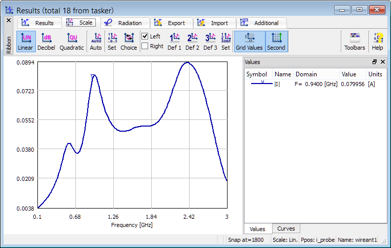
Fig. 2.3.4-5 The FD-Probing post-processing results in wireant1 example: current flowing through i_probe.

There is one more example in the same directory: ..\Antennas\Wireant\wireant1.pro. It shows that the excitation point can be placed directly on the wire, without the necessity of making a gap in the wire. In such a case, the software automatically makes such a gap and places there the lumped source/probe. This feature is convenient when we analyse the same geometry with different meshing: the size of the gap automatically adjusts to the mesh.

In QW-3D up to version 5.0, a point placed on the wire had a different meaning. It did not add any excitation or loading to the structure but instead caused line integration of the four H-field component surrounding the point and Fourier-transforming them. The result was the current flowing in the wire.

This function is obtained in versions 5.0 and up by setting specific constraints on the lumped source/probe placed on the wire: its impedance must be zero, and it must be either a probe or a source of zero amplitude. An additional i_probe is set on the wire in wireant1 to demonstrate this functionality. Since we now have two lumped sources/probes taking part in FD-Probing post-processing, in QW-Simulator we will obtain two separate post-processing results sets. Pressing  button in Results tab allows choosing one of available post-processing results. Let us choose i_probe post-processing results. Current in the wire at i_probe is shown in Fig. 2.3.4-5. It confirms the resonance at 0.940 GHz.

One more post-processing may be demonstrated in wireant1, namely, the display of 3D radiation patterns. Pressing  button in Results tab invokes the 3D Radiation Patterns dialogue on the left of Fig. 2.3.4-6. Its settings produce the pattern shown on the right. Note that 3D radiation patterns calculations are time consuming as they amount to calculating multiple 2D patterns.

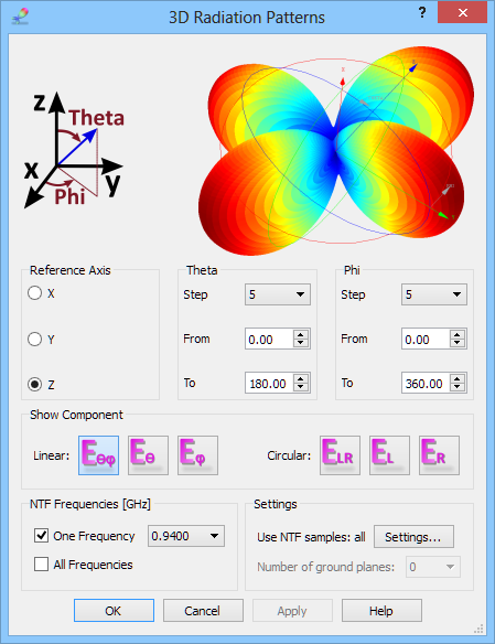
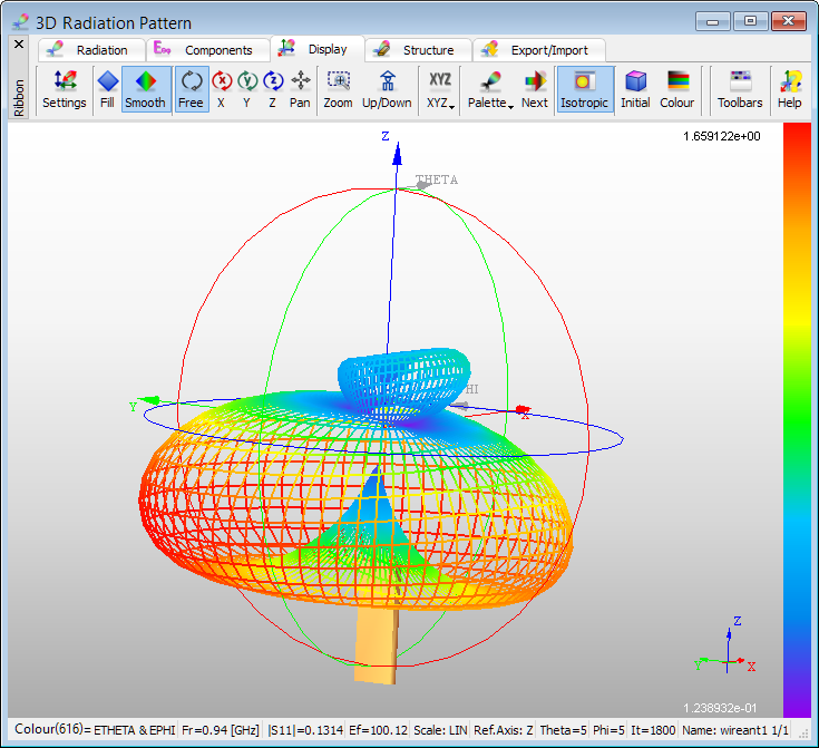
Fig. 2.3.4-6 3D Radiation pattern in wireant1 example.

Fig.UG 2.3.4-7 The results of simulation of the return loss of wireant.pro and wireant1.pro.

Finally, let us compare the S-parameter results of wireant1 and wireant (Fig. 2.3.4-7). The two curves coincide at low frequencies but slightly bifurcate at higher frequencies. This is due to differences in the modelling of radial electric and loop magnetic fields in the source area. In FDTD cells including wires, FDTD equations are modified to take wire diameter and 1/r field behaviour into account. This is also the case when the source is placed on the wire, as in wireant1. When the gap is explicitly cut by the user, as in wireant, the fields around the gap are calculated by standard FDTD equations.