2.15.1 Optimisation of a waveguide-to-coax transition
QW-3D opens a possibility of using an optimiser (named QW‑OptimiserPlus) fully integrated with QW-Simulator. QW-OptimiserPlus uses a new library O2DLL_F developed by Dr. L.J.Opalski and sold as an optional module in QuickWave software family. It matches efficiency and reliability with a new, very user-friendly interface built in the QW-Simulator. Application of QW-OptimiserPlus will be explained here on two examples. Description of its interface in QW-Simulator can be found in QW-OptimiserPlus manual.
Let us start from the example already discussed in this manual - the waveguide- to-coax transition. In QW-Editor open the example Opt_Plus\Wgtocx4\wgtocx4.pro. This example is basically the same as Standard\Various\Wgtocx\wgtocx1.pro example. The only difference is that wgtocx4.pro uses automatic AMIGO meshing option (see Application of AMIGO for reference). In general, using AMIGO is highly recommended for optimisation tasks because it automatically generates meshing close to optimal one and avoids creating small FDTD cells.
In QW-Editor with wgtocx4.pro open, invoke Select Object (![]() button in 2D Window) and double-click over wgtocx4.udo. When the UDO header opens, verify the state of UDO parameters. Note that the name of the UDO object was set to be the same as the name of the project. This is a general requirement for QW‑OptimiserPlus. The optimiser interface of QW-Simulator will modify variables only in the object having the same name as the project.
button in 2D Window) and double-click over wgtocx4.udo. When the UDO header opens, verify the state of UDO parameters. Note that the name of the UDO object was set to be the same as the name of the project. This is a general requirement for QW‑OptimiserPlus. The optimiser interface of QW-Simulator will modify variables only in the object having the same name as the project.
Now press ![]() button from Simulation tab of QW-Editor to run wgtocx4.pro in QW-Simulator. We see the result well known from Waveguide-to-coax transition. We note that about 2000 iterations are needed to obtain well converged results of S11 versus frequency. We press the red light [
button from Simulation tab of QW-Editor to run wgtocx4.pro in QW-Simulator. We see the result well known from Waveguide-to-coax transition. We note that about 2000 iterations are needed to obtain well converged results of S11 versus frequency. We press the red light [![]() ] to stop the simulation, but do not close QW‑Simulator main window. We are ready to prepare the optimisation run (or verify if it has been prepared correctly). We press
] to stop the simulation, but do not close QW‑Simulator main window. We are ready to prepare the optimisation run (or verify if it has been prepared correctly). We press ![]() button in Optimiser tab to open the main dialogue of QW‑OptimiserPlus interface.
button in Optimiser tab to open the main dialogue of QW‑OptimiserPlus interface.
There are three tabs in the dialogue. First we press Preferences. In the upper part of the window we see the path to QW-Editor to be used during optimisation. Default is /qedmute.exe or in other words, the mute version of QW-Editor placed in the qwbin directory. On the right hand side we choose the number of FDTD iterations per simulation. In our example 2000 iterations are sufficient and thus we place that number. We also check View Goal Function Changes to automatically obtain a window monitoring the progress of optimisation during its run.
On the left side of the dialogue we choose the proper stop criteria. They include the Maximum Number of Simulations after which QW-OptimiserPlus stops regardless of other criteria. We have also a choice between two options:
- Stop when Goal Function Reaches G0 (with default value G0=0). The goal function drops down below zero when the objectives are within the requested bounds. Thus it is natural to stop the simulation at that point and we accept it.
- Stop when Goal Function Stabilises with Tolerance GT with (with default value GT =1e-6). When this option is activated, the progress of goal function is monitored and the process stops when several best results fall within the GT margin suggesting that no progress can be made beyond that point.
Electromagnetic simulations often produce goal functions with many minima and rather rough (or we can say noisy). This can be confusing for the criterion based on goal function tolerance, often used for other applications of optimisers. On the other hand, the design engineer usually knows well what his goals are. That is why we think that the option to “try hard” without stopping when the goal function stabilises seems to be more practical in most applications of QW-3D. However, we leave the other option for the user’s decision. Later in this Section we will exemplify the consequences of that choice when running wgtocx4 example.
There are also some advanced options of using theQW-OptimiserPlus which we shall not modify in the considered example. They are explained in Preferences and the user is encouraged to try and run this example later with modified advanced parameters to see how they affect the optimisation process.
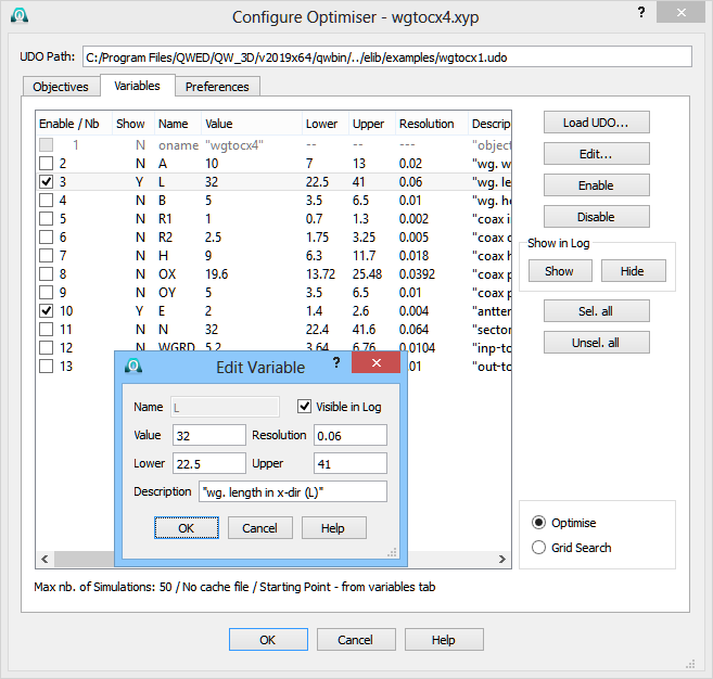
Fig. 2.15.1-1 Configure Optimiser dialogue for wgtocx4 example with open Edit Variable dialogue for variable L.
Now we switch to the Variables tab. In the upper part of the window we can see the path to the *.udo file from which variables and their defaults have been read. This should be the same file from which the object in the project has been created. The dialogue (Fig. 2.15.1-1) shows the list of variables of the considered object. Any numerical ones can be chosen here as optimisation variables (enabled). Actually, two of them (L and E) are shown to be chosen. The line of variable L is highlighted and thus we can press ![]() to modify its settings also shown in Fig. 2.15.1-1. We can set the initial value for optimisation as well as its lower and upper constraints. We also decide if its current value should be displayed in the Optimisation Log during the optimisation process. Moreover, we can define its resolution. The resolution of 0.06[mm] means that the user expects that modification of L by less than resolution will be insignificant for the goal function. Thus the QW-Optimiser will not run additional electromagnetic simulation when the optimisation procedure suggests that the value of L should be changed by less than 0.06 mm with respect to one of the already calculated points. This is supposed to save computing time but too high resolution may limit the ability of the optimisation procedure to reach its precise optimum.
to modify its settings also shown in Fig. 2.15.1-1. We can set the initial value for optimisation as well as its lower and upper constraints. We also decide if its current value should be displayed in the Optimisation Log during the optimisation process. Moreover, we can define its resolution. The resolution of 0.06[mm] means that the user expects that modification of L by less than resolution will be insignificant for the goal function. Thus the QW-Optimiser will not run additional electromagnetic simulation when the optimisation procedure suggests that the value of L should be changed by less than 0.06 mm with respect to one of the already calculated points. This is supposed to save computing time but too high resolution may limit the ability of the optimisation procedure to reach its precise optimum.
Now we switch to the Objectives tab. In the considered example we have one objective, which will be better explained in the dialogue obtained after pressing ![]() (Fig. 2.15.1-2). On the left side we can chose the type of post-processing on which the goal function will be defined. In general, we have the choice of Scattering Parameters, Radiation Patterns, FD-Probing, Scattering SMN Parameters or Saved Data. In the considered example the only choices are S11 or S21. We choose |S11| to be optimised for minimum in a defined frequency range. We set our target value to T=0 and the upper bound to UB=0.1. This means that |S11|<0.1 is a satisfactory solution and the goal function will be calculated as:
(Fig. 2.15.1-2). On the left side we can chose the type of post-processing on which the goal function will be defined. In general, we have the choice of Scattering Parameters, Radiation Patterns, FD-Probing, Scattering SMN Parameters or Saved Data. In the considered example the only choices are S11 or S21. We choose |S11| to be optimised for minimum in a defined frequency range. We set our target value to T=0 and the upper bound to UB=0.1. This means that |S11|<0.1 is a satisfactory solution and the goal function will be calculated as:
G = Max (O-UB)/(UB-T)
where O is the maximum value of |S11| in the considered Sub-Range. The solution is satisfactory when the goal function drops below zero.
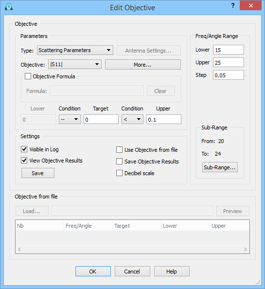
Fig. 2.15.1-2 Edit Objective dialogue in wgtocx4 example.
Frequency range and sub-range are defined on the right side of the Edit Objective dialogue. First we need to set the proper Frequency Range and step of the post-processing. (Attention: they must be identical with those defined in QW-Editor for the relevant post-processing). Now we press ![]() to obtain the dialogue of Fig. 2.15.1-3. Here we can set the subrange for the considered objective. We have chosen the Sub-Range from 20 to 24 GHz. In that range each of the frequency points (calculated by QW-Simulator with a step of 0.05 GHz) will be considered for calculation of the Goal Function.
to obtain the dialogue of Fig. 2.15.1-3. Here we can set the subrange for the considered objective. We have chosen the Sub-Range from 20 to 24 GHz. In that range each of the frequency points (calculated by QW-Simulator with a step of 0.05 GHz) will be considered for calculation of the Goal Function.
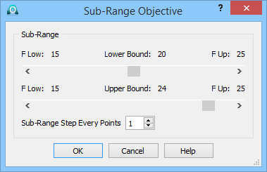
Fig. 2.15.1-3 Setting Sub-Range in wgtocx4 example.
Now we press OK to upload the current settings of the Configure Optimiser dialogue. The software is ready to run the optimization. If the example is being optimised for the first time, we have no formerly calculated results stored in Optimiser Cache. If this is not the first run, we should decide whether we want QW-OptimiserPlus to use earlier experience about the example stored in its Cache. If not, we should invoke clear the Cache by pressing ![]() button and the optimisation process will start from scratch. Basically, the cache has to be cleared when objectives have been added or deleted in the Configure Optimiser dialogue or the project has been changed in QW-Editor.
button and the optimisation process will start from scratch. Basically, the cache has to be cleared when objectives have been added or deleted in the Configure Optimiser dialogue or the project has been changed in QW-Editor.
We press ![]() button and the optimisation process starts. Its progress is recorded in the Optimiser Info tab of Simulator Log. Asterix at the beginning of the line (e.g. *Opt=3) means that the goal function value calculated in that run is the smallest one so far. After the first simulation is completed, QW-Simulator opens two more windows. In one of them the calculated |S11| is shown. Five curves are displayed at a time, indicating the first, the last and best of the obtained results as well as Target and Upper bound of the objective. In the other window, the goal function versus the number of optimisation iterations is presented. After 45 steps the optimisation stops indicating that: Target objective function value reached.
button and the optimisation process starts. Its progress is recorded in the Optimiser Info tab of Simulator Log. Asterix at the beginning of the line (e.g. *Opt=3) means that the goal function value calculated in that run is the smallest one so far. After the first simulation is completed, QW-Simulator opens two more windows. In one of them the calculated |S11| is shown. Five curves are displayed at a time, indicating the first, the last and best of the obtained results as well as Target and Upper bound of the objective. In the other window, the goal function versus the number of optimisation iterations is presented. After 45 steps the optimisation stops indicating that: Target objective function value reached.
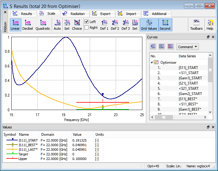

Fig. 2.15.1-4 Results of optimisation of wgtocx4 example.
Let us look at |S11| obtained during the analysis (Fig. 2.15.1-4). Indeed the Goal Function has dropped below zero and the reflections are lower than 0.1 (-20 dB) in the entire subband of interest.