2.10.1   Basic example of application of DXF Converter

The  button in Model tab and Tools->DXF Converter command from main menu of QW-Editor invoke file open dialogue for *.dxf file and next DXF Converter Options dialogue that allows setting conversion parameters (Fig. 2.10.1-2).

Let us consider an example stored as ..\Filters\Msfilter\msfilter.pro. This project is ready to run. However, here we will assume that it is being built from scratch, based on the available msfilter1.dxf file. The msfilter1.dxf has been prepared under another CAD software package, and describes a microstrip filter geometry shown in Fig. 2.10.1-1.

Thus we will start a new QW-3D project ..\DXF\Msfilter\msfilter1.pro and try to import msfilter1.dxf using DXF Converter available in QW-Editor.

Please open QW-Editor and load ..\DXF\Msfilter\msfilter1.pro. It is an empty project with two 2D and 3D Windows as in the original msfilter.pro.

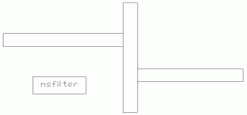
Fig. 2.10.1-1 View of msfilter1.dxf file.

Open Circuit dialogue (by pressing  button in the Model tab) and choose Air as a default medium.

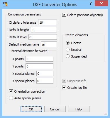
Fig. 2.10.1-2 DXF Converter Options dialogue.

Now click over  button in Model tab and browse the example directories to find and open ..\DXF\Msfilter\msfilter1.dxf. Then the DXF Converter Options window with the default options will appear on the screen, as shown on Fig. 2.10.1-2.

Let us explain the meaning of the DXF Converter Options shown in the window of Fig. 2.10.1-2:

·       Delete previous object – a typical setting, which means that the software will delete all objects previously stored under the same name as the new object(s) to be created from *.dxf file.

·       Circle/Arc tolerance – a circle or an arc is approximated by a regular polygon with the number of vertices defined by the user. A higher number of vertices gives better accuracy but slows down QW-Editor operations. The recommended number is from 16 to 64.

·       Default height – here we can set the height of all 2D elements converted from *.dxf file. The elements already declared in *.dxf file as 3D have their own height, which supersedes the default height of DXF Converter.

·       Default level – the level in the QW-Editor project whereat the obtained object is based.

·       Default medium name – this medium will be automatically assigned to all the elements generated as a result of conversion from *.dxf file. (Later the media of individual elements can be manually changed).

·       Minimal distance between:

§  X points – snap to X point - sets a minimum distance between X-coordinates of neighbouring points. If the distance between two points in the X-direction is smaller than this snap, then the X-coordinate for point2 will be made equal the X-coordinate for point1. This and the next option are used to repair minor errors of *.dxf files resulting in unintentional microscopic slots or overlapping of two elements.

§  Y points – snap to Y point – similar as above but for the Y-coordinate.

§  X special planes – sets a minimum distance between neighbouring X=const mesh snapping planes, automatically generated during the conversion. If the distance is smaller than the setup value, then the second mesh snapping plane will be ignored. Note that the Auto special planes option needs be checked for mesh snapping planes to be automatically generated at all.

§  Y special planes – similar as above but for the Y-coordinate.

·       Orientation correction – in QW-3D the circumference of the elements should be left (counter-clockwise) oriented. This option is used for automatic correction of all the elements converted from the *.dxf file, if they are right (clockwise) oriented.

·       Auto special planes – if checked, mesh snapping planes will be automatically added where necessary.

·       Create elements - this toggle determines the positions of the bottoms and covers of all converted elements with respect to the FDTD mesh:

§  Electric – E-planes of the FDTD grid (see FDTD method in QuickWave Software) will be enforced at all bottoms and covers.

§  Neutral – either an E-plane or an H-plane will be enforced at each bottom or cover.

·       Suppress info – if not checked, the progress of *.dxf file conversion will be displayed.

·       Create log file – if checked, the information about conversion will be saved in a text file in the same directory as the *.dxf file (for example if the *.dxf file is: c:\dxf\msfilter1.dxf, log file will be: c:\dxf\msfilter1.txt).

Now press OK to convert msfilter1.dxf with the default options of Fig. 2.10.1-2. A black window appears on the screen for a while. Eventually we obtain the view shown on Fig. 2.10.1-3.

Note that two new files have appeared next to msfilter1.dxf (in the same directory). The msfilter1.udo file contains the structure from *.dxf file described in the UDO language; it is always created after conversion. The msfilter1.txt file contains information about the conversion process; it is created only if Create log file option is checked.

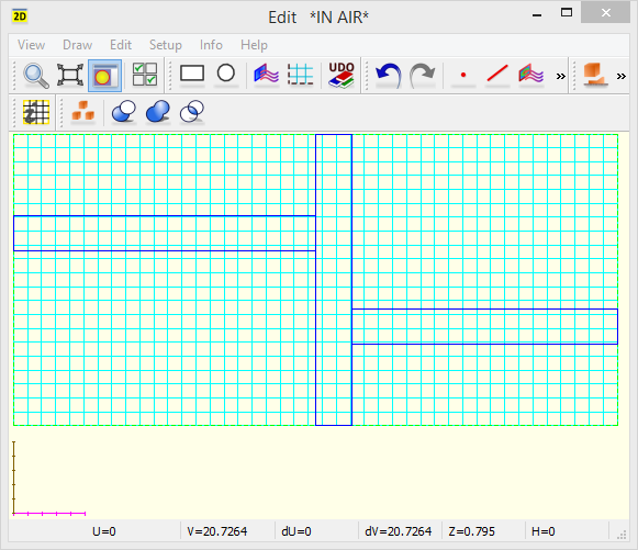
Fig. 2.10.1-3 The microstrip filter metallization shape in QW-Editor after conversion from msfilter1.dxf file with the default options of DXF Converter as in Fig. 2.10.1-2.

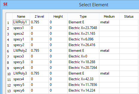
Press the Select Element  [] button to see the list of elements:

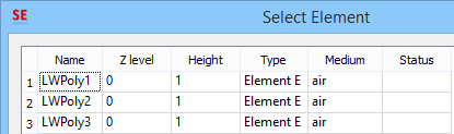
Note that all elements are based at the default level 0, have a default height 1, and are filled with a default medium air.

If you have difficulties in associating the three elements with the appropriate parts of the structure, please try to highlight one element on the Select Element list, and then Mark it. It will appear in the graphical display with a thick contour line. Applying such a procedure, we have located the three elements within the structure, as presented in Fig. 2.10.1-4.

The circuit described by the msfilter1.dxf file (Fig. 2.10.1-1) and the circuit obtained after conversion (Fig. 2.10.1-3) are somewhat different because DXF onverter can convert only elements described by their geometry. The elements apparently missing in Fig. 2.10.1-3 are those, which in DXF format have not been described by their coordinates. In this particular case, the text box has been ignored by DXF onverter.

Let us now demonstrate the influence of Minimal distance between: X points and Y points options. In Fig. 2.10.1-3 we can see the circuit after conversion in the case when these options have been effectively off (since, as shown in Fig. 2.10.1-2, the minimal distance has been 0). Fig. 2.10.1‑5 shows the enlargement of the region (marked as a black rectangle in Fig. 2.10.1‑4), where the X coordinates should physically be the same, but they have not been the same in the *.dxf file.

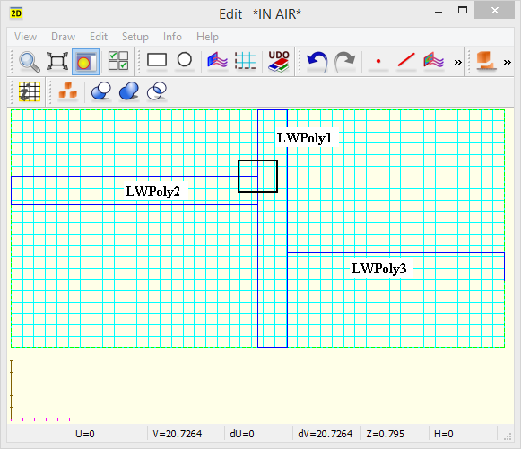
Fig. 2.10.1-4 Element names associated with consecutive elements generated from msfilter1.dxf file.

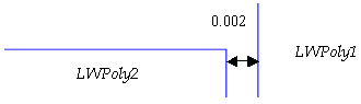
Fig. 2.10.1-5 Unintentional slot to be corrected using Minimal distance between: X points option.

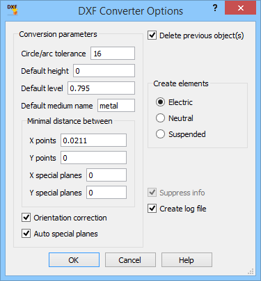
Fig. 2.10.1-6 DXF Converter Options dialogue window with the setting appropriate for msfilter1.dxf conversion.

Let us now repeat the conversion process from the beginning but with the DXF Converter Options as shown in Fig. 2.10.1-6. We have changed the default level to 0.795, the default height to 0, the default medium to metal. We have also set Minimal distance between: X points to 0.0021, and activated Auto special planes. The result is presented in Fig. 2.10.1-7. Using Zoom function we can check that the gap between the elements has vanished (see Fig. 2.10.1-8). Moreover, mesh snapping planes have been added to enhance the modelling of metal edges (green lines in 2D Windows of QW-Editor).

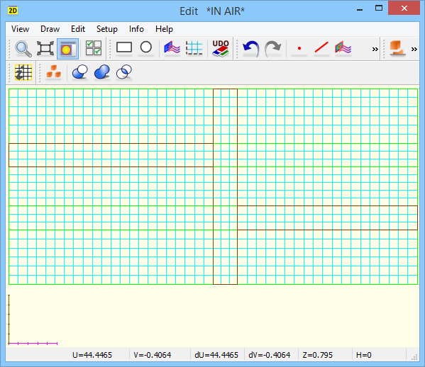
Fig. 2.10.1-7 Strip of the microstrip filter in QW-Editor after conversion from msfilter1.dxf file withDXF Converter options as in Fig. 2.10.1-6.

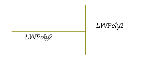
Fig. 2.10.1-8 Effect of using snap to point (Minimal distance between: X points and Y points options).

Now press  button to see the list of elements and automatically added mesh snapping planes:

Pressing Select Object [] reveals that an object msfilter1.udo has been created. Double click on its name invokes its header as shown in Fig. 2.10.1-9, where we can conveniently modify the parameters.

Fig. 2.10.1-9 Msfilter1.udo created as a result of conversion from msfilter1.dxf file.

Let us now take a look at the structure of conversion log in msfilter1.txt file:

----------------------------------------------------------

DXF2UDO converter version v2.1: 2009.09.08

C:\Program Files\QWED\QW_3D\v2015x64\envir\..\qwbin\dxf2udo.exe -n C:\Users\Public\QWED\v2015x64\qw_examp\QW_3D\DXF\Msfilter\msfilter1.dxf -a 16 -L 0.795 -h 0 -m metal -k e -x 0.0021 -y 0 -X 0 -Y 0 -l -s -c -S  s -c -S 

   Circle/Arc Tolerance: 16

   Height: 0.000000

   Level: 0.795000

   Medium: "metal"

   Element kind: INe

   Bi-Phase: No

   Left Oriented Correction: Yes

   Auto Special Planes: Yes

   Snap2Point X: 0.002100

   Snap2Point Y: 0.000000

   Min. dist. X sp. pl.: 0.000000

   Min. dist. Y sp. pl.: 0.000000

Date: Fri Sep 23 14:34:21 2011

Filename: C:\Users\Public\QWED\v2015x64\qw_examp\QW_3D\DXF\Msfilter\msfilter1.dxf

  ENTITIES 1 Section found

      LWPOLYLINE 1 found

            CORNER 1 found

            CORNER 2 found

            CORNER 3 found

            CORNER 4 found

            CORNER 5 found

      LWPOLYLINE 2 found

            CORNER 1 found

            CORNER 2 found

            CORNER 3 found

            CORNER 4 found

            CORNER 5 found

      LWPOLYLINE 3 found

            CORNER 1 found

            CORNER 2 found

            CORNER 3 found

            CORNER 4 found

            CORNER 5 found

      ! INSERT found - UNKNOWN COMMAND

      ! INSERT found - UNKNOWN COMMAND

      ! TEXT found - UNKNOWN COMMAND

  ENTITIES 1 End Section

  SUMMARY:

      LWPOLYLINE 3 found

      [LINES]  0

      [OTHERS] 3

End of File: C:\Users\Public\QWED\v2015x64\qw_examp\QW_3D\DXF\Msfilter\msfilter1.dxf UDO File Parameters 0/3

   LWPOLYLINE 1 - Left Oriented Correction

   LWPOLYLINE 1 - Zero Length Correction

   LWPOLYLINE 1 - Special Planes (X/Y) 2/2              

   LWPOLYLINE 2 - Snap2Point (X/Y) 2/0              

   LWPOLYLINE 2 - Left Oriented Correction

   LWPOLYLINE 2 - Zero Length Correction

   LWPOLYLINE 2 - Special Planes (X/Y) 1/2              

   LWPOLYLINE 3 - Snap2Point (X/Y) 3/0              

   LWPOLYLINE 3 - Zero Length Correction

   LWPOLYLINE 3 - Special Planes (X/Y) 1/2              

UDO File Body 0/3              

UDO File Special Planes (X/Y) 4/6              

Date: Fri Sep 23 14:34:21 2011

----------------------------------------------------------

At the beginning of the conversion log file we can see the command line and the conversion options. The following part lists the commands found in the analysed *.dxf file. Some of those do not describe the geometry of the elements and therefore have been marked as UNKNOWN for DXF converter. The SUMMARY section informs about the number of the found elements. At the end of the file we can read a record of repair options applied to the elements. For example, the LWPOLYLINE2 element has been corrected as follows:

·       Snap2Point – the Minimal distance between: X points option has been used and two X-coordinates have been corrected.

·       Left Oriented Correction – the original *.dxf file this element was right (clockwise) oriented; it has been corrected to the left-orientation.

·       Zero Length Correction – at least two consecutive points had the same coordinates in the original *.dxf file; the second point has been ignored.

·       Special Planes – one mesh snapping planeperpendicular to the X-axis and two mesh snapping planes perpendicular to the Y-axis have been automatically generated by DXF converter.

So far we have imported the strip layout available in msfilter1.dxf file. We need several other steps to make the project complete for running. First we must declare the dielectric substrate of permittivity 2.2. Please open Project Media dialogue and add a new medium called diel with Eps=2.2.

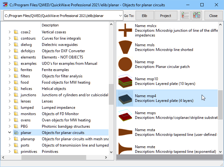
Fig. 2.10.1-10 UDO library window showing the list of available libraries.

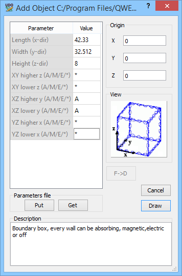
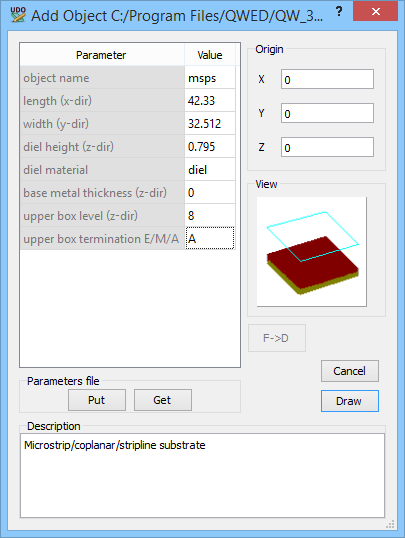
Fig. 2.10.1-11 The header of msps.udo.                                     Fig. 2.10.1-12 The header of bbox.udo.

Now we need to draw the substrate for our microstrip filter. We shall refer to the powerful UDO library, where we can certainly find the substrate appropriate for simulations. Press  button in the 2D Window; the window like in Fig. 2.10.1-10 will appear. Select the appropriate library, which in our case is planar. Click its name. Now we can see all the objects available in the Planar UDO library. Please click over the msps.udo and set in its header the parameters presented in Fig. 2.10.1-11; then press Draw.

What remains to be done is the introduction of the side absorbing walls. We could do this manually. However, it is more convenient to use ..\boxes\bbox.udo, designed to draw any or all of the boundaries surrounding a cuboidal box. We choose only two Y-plane absorbing sides (see Fig. 2.10.1-12) since the upper absorption has already been drawn using msps.udo, the lower boundary is metal ground plane, and X-sides will be transmission line ports.

Let us now introduce the ports. First we introduce the input port. We press  button in the 2D Window and select the ports library. Please click over the portoxe.udo. Set the parameters as shown on the left hand side of Fig. 2.10.1-13 and press OK. Then repeat the operation for the output port setting the parameters as shown in the right part of Fig. 2.10.1-13.

In msfilter.pro there is a special (mesh snapping and modifying) plane at Z=2.5, so for the agreement with the original project let us introduce it in msfilter1.pro. Invoke Special Planes and Boundaries dialogue ( button). Select Z Orientation and introduce Position 2.5; press Insert and press Cancel. Press  and double click on the Z special plane. Now press right mouse button, set Forced cell size-Plus to 1 and press OK.

Now we will set the mesh. Press  button in 2D Window and set 0.5 for X, 0.5 for Y and 0.3 for Z direction, respectively; press OK.

Further parameters of the simulation are defined through the Edit Transmission Line Port (under  button in Model tab) and S-Parameters  (under  button in Simulation tab) dialogues. Both can also be accessed by shortcut buttons in the main toolbar of QW‑Editor.

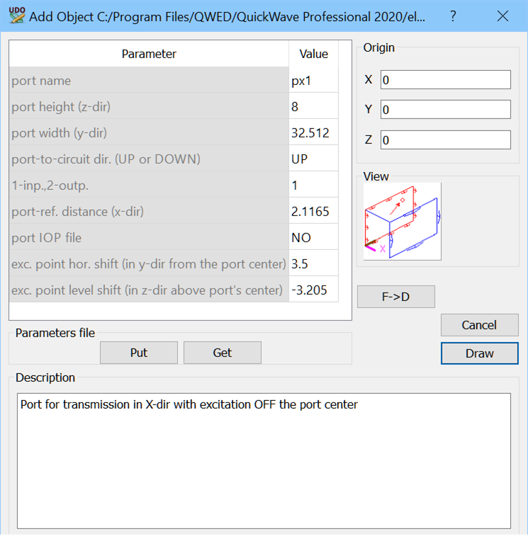
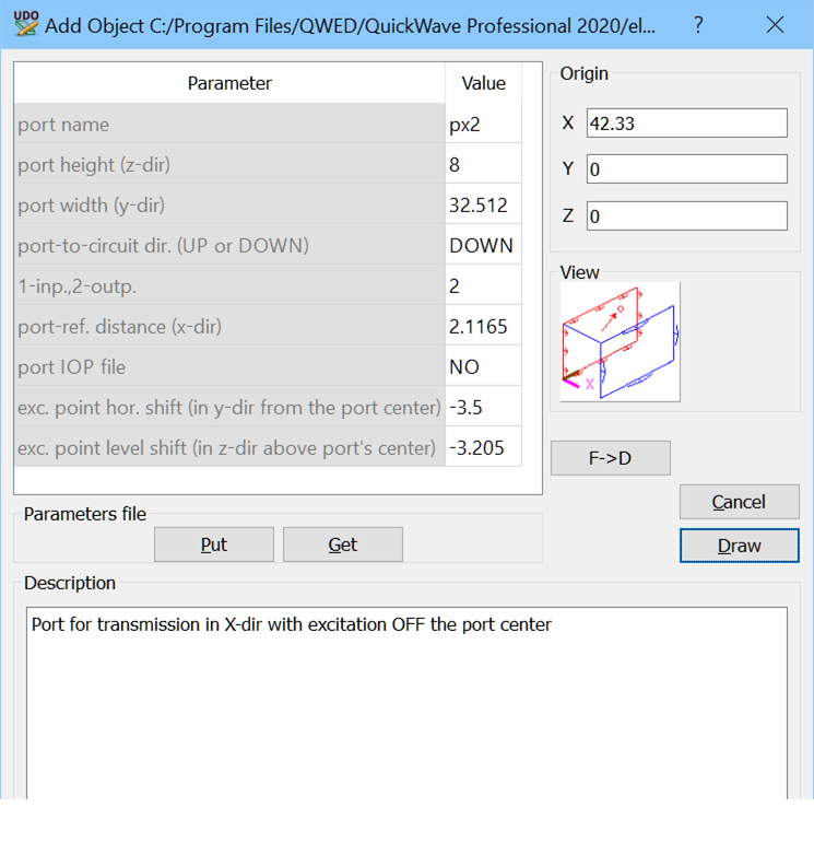
Fig. 2.10.1-13 The header of portoxe.udo with appropriate settings for input port (left) and output port (right).

Open Edit Transmission Line Port dialogue for source and load ports to set their parameters. For input port (called px1):

·       Select Exciting field as TEM.

·       Select Excitation Waveformas pulse of spectrum f<f2

·       Set spectrum limit f2=20 GHz;

For output port (called px2):

·       Select Exciting field as TEM.

·       Select Excitation Waveformas pulse of spectrum f<f2

·       Set spectrum limit f2=20 GHz;

Open S-Parameters dialogue:

·       activate the S-Parameters post-processing

·       set the frequency range: from 0 GHz to 20 GHz step 0.1 GHz

To start calculations press  button in Simulation tab of QW-Editor. After about 2500 iterations suspend the simulations using  button in Run tab of QW-Simulator. Actually, it may be impossible to press  exactly at the 2500^th iteration because the iterations will be running too fast. In such a case, please press  earlier and perform the remaining steps by consecutively pressing  button.

Actually, a more convenient approach to suspending the analysis at a specific iteration is by using the Breakpoints mechanism. If the simulation is running, stop it using  button; if you are still in QW-Editor, launch the QW-Simulator using  button. Press  button in Run tab of QW-Simulator to open Breakpoints dialogue. Press Add button and choose Suspend command from Other Commands. Set the desired iterations (2500 here) in the Iteration field, press OK in the Add Breakpoint dialogue and OK in the Breakpoints dialogue.

After the simulation is suspended, open the Results window by pressing  button in Results tab of QW-Simulator. For further comparisons, please save the results using  button available in Export tab of Results setting the file name as msfilter1_s.da3.

Fig. 2.10.1-14 Compared results obtained with the original project msfilter.pro (blue curve) and with the new project msfilter1.pro (green curve) prepared using msfilter1.dxf file and standard library objects.

Now in QW-Editor open the original msfilter.pro and press . Suspend simulation after 2500 iterations and press  button in Results tab to see the simulation results. To compare these results with the results for msfilter1.pro press  button in Import tab of Results window and choose msfilter1.da3 file saved before.

Both results are identical, as shown in Fig. 2.10.1-14. This confirms that you have correctly reconstructed msfilter1.pro by importing msfilter1.dxf!