2.1 Simple horn antenna
The horn antenna with one corrugation is stored in the ..Antennas/Ant1/ant1.pro file in the installation.
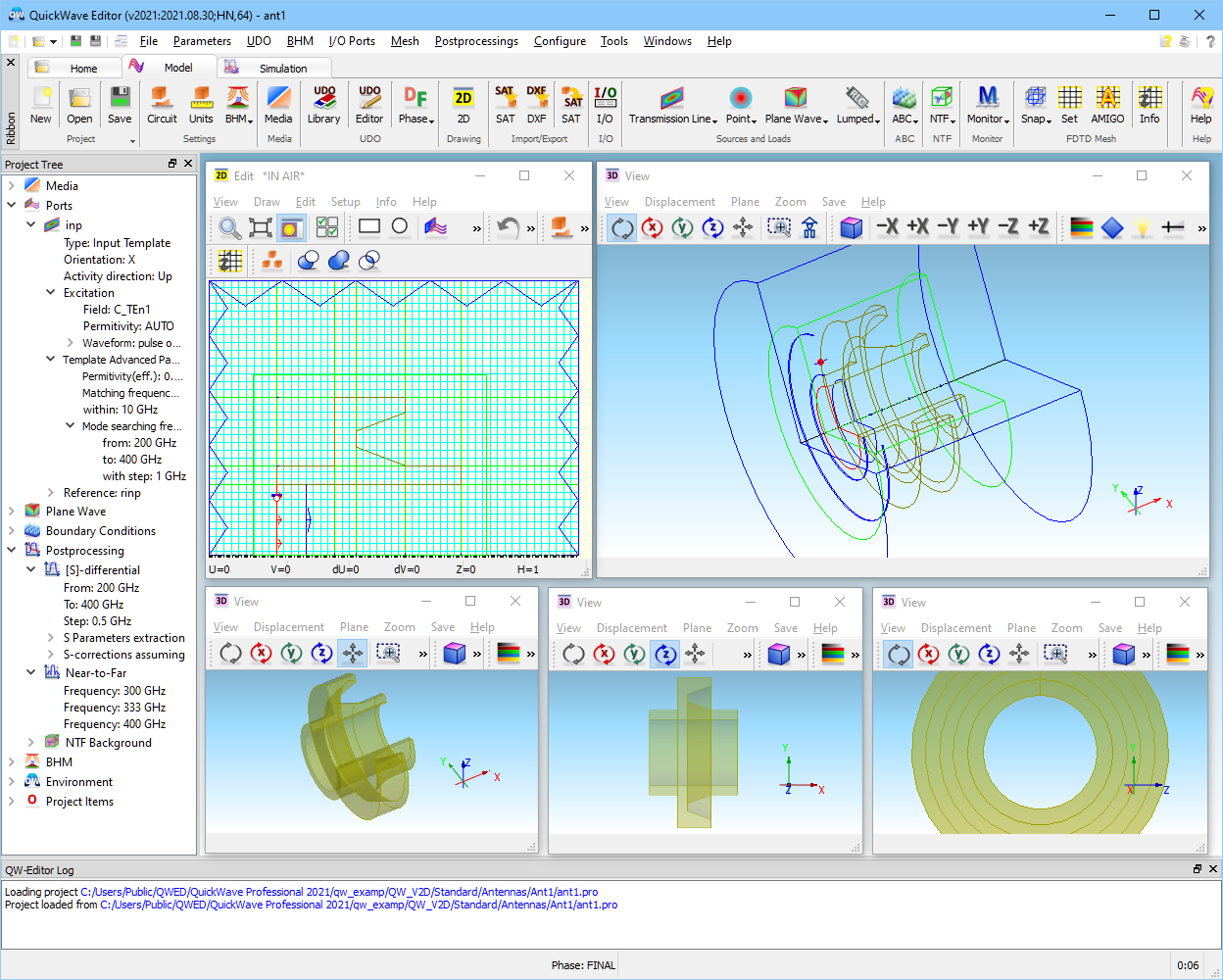
The views of the antenna structure in QW-Editor have been given in Fig. 2.1-1.
Fig. 2.1-1 The screen with displayed ant1 project.
Press the ![]() button (or equivalently the File-Export & Run-Export, Run & Start command from main menu). QW‑Simulator completes the template generation stage (as described in Template mode generation procedure) and starts the analysis of the antenna. Open the Results window for S-parameters results in Cartesian coordinates
button (or equivalently the File-Export & Run-Export, Run & Start command from main menu). QW‑Simulator completes the template generation stage (as described in Template mode generation procedure) and starts the analysis of the antenna. Open the Results window for S-parameters results in Cartesian coordinates ![]() to first see how the return loss is being extracted. Note that the display of QW‑Simulator results is controlled by the contents of environment file, if it exist:
to first see how the return loss is being extracted. Note that the display of QW‑Simulator results is controlled by the contents of environment file, if it exist:
· ant1.en8: If the ant1 example has been previously analysed, and the S-parameter results have been displayed (in one or more windows), the description of successive windows (layout, scale, number and type of displayed curves) has been saved in the file ant1.en8. Those windows will now be successively reproduced, upon the opening of successive Results windows.

Fig. 2.1-2 Return loss amplitude of the ant1 example, after 5000 iterations, in program default settings.
When you first run ant1.pro after installing QW-V2D, ant1.en8 in its installation version will be used. The Results window for S-parameters results will display the |S11| curve in the window in manual decibel scale. After 5000 iterations we will see the display as in Fig. 2.1‑2. The contents of the window practically stabilise at this stage. Invoke the Suspend command in the Run tab to suspend the FDTD simulation.
We can modify the scale of display via the Set command (or Ctrl+S) in the Scale tab of Results window. The Scaling dialogue appears. As shown in Fig. 2.1-3, it offers two basic ways of scale modification. The first is to have scaling type as manual, and to introduce the maximum, minimum and step values. The other is to choose one of the pre-defined scales from the list available at the bottom of the dialogue.
We press OK with the settings shown in Fig. 2.1-3. We obtain the |S11| curve as in Fig. 2.1-4. At 300 GHz we find the return loss of 0.1030.
Pressing N on the keyboard (or Setup-Switch-Next) changes the display to the S11 phase, which will be assigned to the right scale and shown in Auto scale.
Pressing N again changes the display to the absolute value of the propagation constant. It will not be visible in the left ScaleY (vertical) set for the |S11|. We may either change the scale again, or open another Results window for S-parameters results to get Fig. 2.1-5. The user is recommended to take a look at this curve when he first runs a particular project, since it permits to immediately verify if a correct mode has been applied at the input. The curve of Fig. 2.1-5 shows a cut-off frequency at approximately 246.5 GHz, as expected for the TE11 mode in our guide.

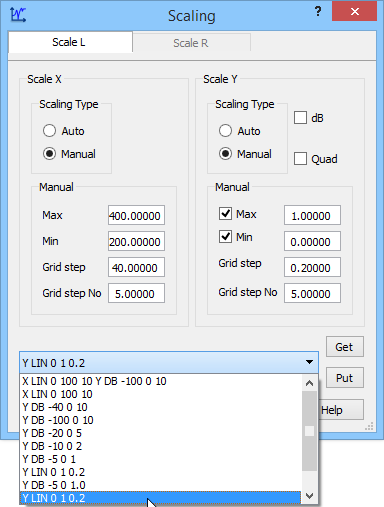
Fig. 2.1-3 Scaling dialogue used to define the scale manually (upper) or to select it from the list (lower).
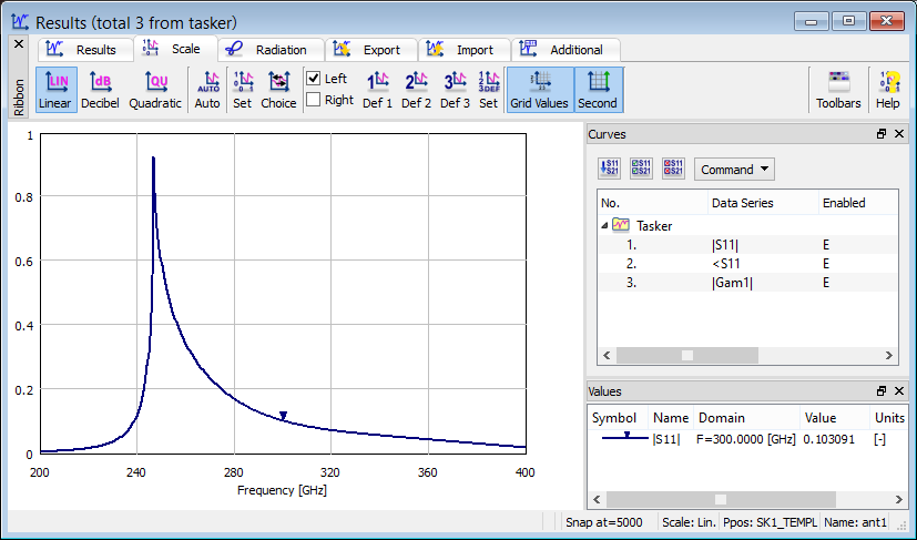
Fig. 2.1-4 Return loss amplitude of the ant1 example, after 5000 iterations, with scaling as in the upper part of Fig. 2.1-3.
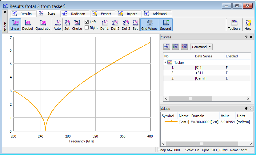
Fig. 2.1-5 Display of propagation constant versus frequency in the input guide of the ant1 example, after 5000 iterations.
To see the calculated radiation patterns, open Results window for 2D radiation pattern by pressing ![]() button (alternatively, you can switch to the NTF post-processing by pressing Postprocessing button in Run tab, what switches the active post-processing to the next one on the list, and then press Results button in the Results tab of QW-Simulator). We will obtain the Radiation Patterns dialogue of Fig. 2.1-6. It proposes the settings of:
button (alternatively, you can switch to the NTF post-processing by pressing Postprocessing button in Run tab, what switches the active post-processing to the next one on the list, and then press Results button in the Results tab of QW-Simulator). We will obtain the Radiation Patterns dialogue of Fig. 2.1-6. It proposes the settings of:
· Theta Step - 2 degree step in theta angle;
· From..to indicates that the full 0..180 degree angle range is of interest;
· Reference Point - x-coordinate of the reference point at half-length of the NTF box;
· Single radiation pattern has been chosen and Radiated Power calculated from NTF Fields option is automatically activated by the software– calculation of radiated power for gain scaling in the near zone, by integration of the Poynting vector over the NTF box,
· Directive gain scaling.
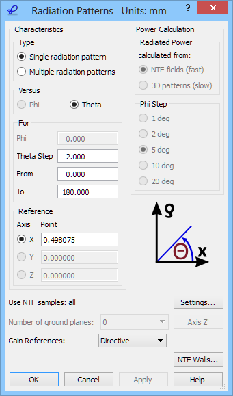
Fig. 2.1-6 The Radiation Patterns dialogue (x,y,z stand for x,r,j directions).

Fig. 2.1-7 Display of Directive gain versus angle of the ant1 example, extracted after 5000 iterations.
Pressing OK with the settings of Fig. 2.1-6 produces the window with radiation pattern results of Fig. 2.1-7. Withant1.en8 settings we see the Etheta and Ephi amplitudes at 300 GHz in manual scale. The window status provides some additional information such as frequency corresponding to the displayed results (300 GHz), radiated power (1.04054 W), and radiation efficiency (100.33 %). The last result has two implications. Firstly, it shows that all power delivered to the antenna through the waveguide feed has been radiated through the NTF boundary. This confirms that convergence has been reached. Secondly, it shows that the error in energy integration may be of the order of 0.3%. This error results from corrections for field averaging at the back NTF surface (at –X direction), applied when Correction for Backward Radiation for V2D projects option in Preferences dialogue from Configure main menu is active (it is active by default). When this option is deactivated the error is 0.001%.
Note that by pressing ![]() button in Radiation tab of the Results window for 2D radiation pattern, the dialogue window of Fig. 2.1-6 with current parameters can be obtained.
button in Radiation tab of the Results window for 2D radiation pattern, the dialogue window of Fig. 2.1-6 with current parameters can be obtained.
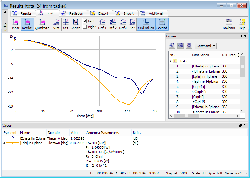
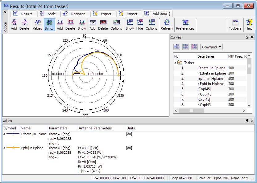
Fig. 2.1-8 Examples of customised displays of radiation pattern results of the ant1 example. Upper display has been obtained from that of Fig. 2.1-7 by using Set option in Scale tab. Lower display has been obtained from the top one by pressing Polar button in Results tab.
We can change scale to decibel via Decibel option in Scale tab (or Ctrl+O). Similarly as in the case of return loss results, we can also use Set option in Scale tab (or Ctrl+S). After setting for the Y-coordinate Max=+10dB, Min=-30dB, Grid Step=8dB we obtain the upper display of Fig. 2.1-8. Pressing Polar button in the Results tab (or Alt+P) changes this to the lower display of Fig. 2.1-8. Clicking the XY button in the Results tab (or Alt+X) causes a change back to the upper display of Fig. 2.1-8.
Enter the Config dialogue by pressing the Config button in Results tab, select the |Copl45| and |Cxpl45| curves and press Show to see the display of Fig. 2.1‑9 (the same can be made by selecting those curves in the Curves frame on the right side of the Results window).
To return to linear scale, press Linear button in Scale tab or press Alt+I (or Setup-Scale-Type-Linear command of main menu).
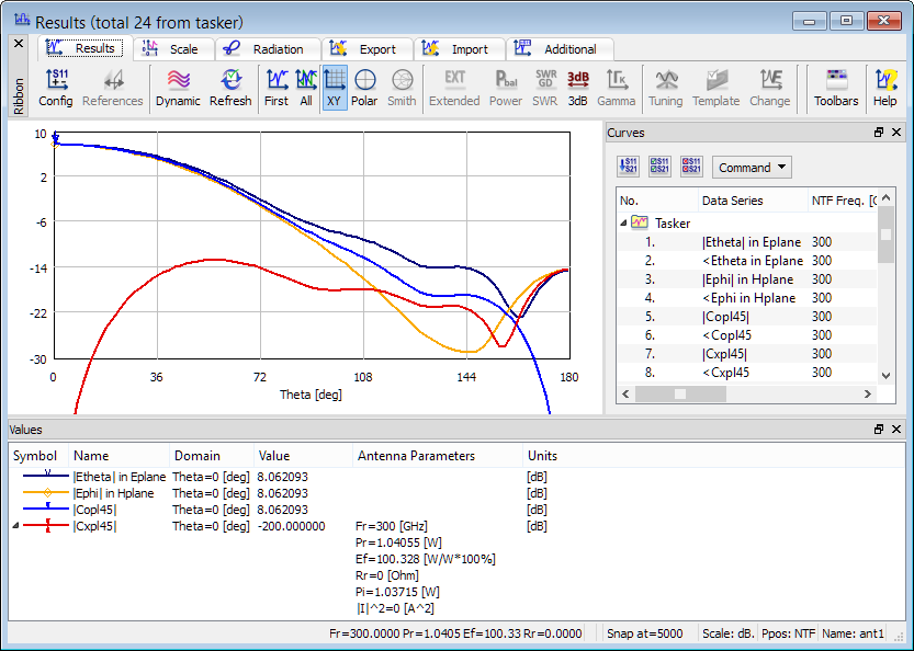
Fig. 2.1-9 The display of radiation patterns including copolar and crosspolar characteristics.
The possibility to show many characteristics in distinctive colours can be exploited in various ways. For example, let us recall that the radiation patterns are simultaneously calculated at three frequencies, defined in the Near to Far dialogue of QW-Editor. In the default operation of QW‑Simulator, the results are displayed for one frequency at a time, and switching between the frequencies is accomplished by pressing Freq. button in Radiation tab or via the Setup-Antenna Settings-NTF freq. command of main menu.
As an alternative, we can use the Config dialogue. The dialogue shown in Fig. 2.1-10 appears. It shows that the calculations of amplitudes and phases of Etheta and Ephi at three frequencies are enabled (which means that each of these characteristics can be displayed by pressing F and/or N buttons), and that the currently visible curves are |Etheta| and |Ephi | at the first frequency. Let us assume that instead of these two, we want to see the three |Etheta| curves at all three frequencies. We highlight this new selection, as shown in the right part of Fig. 2.1-10, and press Show Sel. button. We obtain the bottom display of Fig. 2.1-10 .
Note that since the curves correspond to different frequencies, the information on frequency, radiated power, and efficiency has been moved from the window status to the listing in its right part.
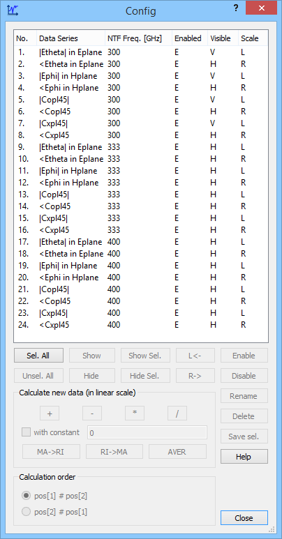
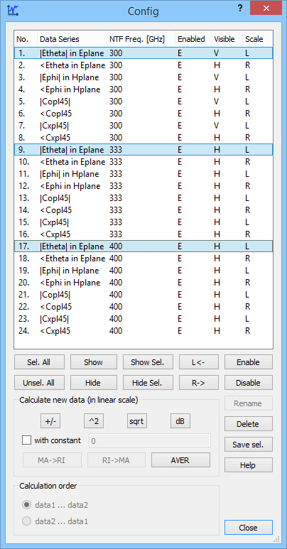
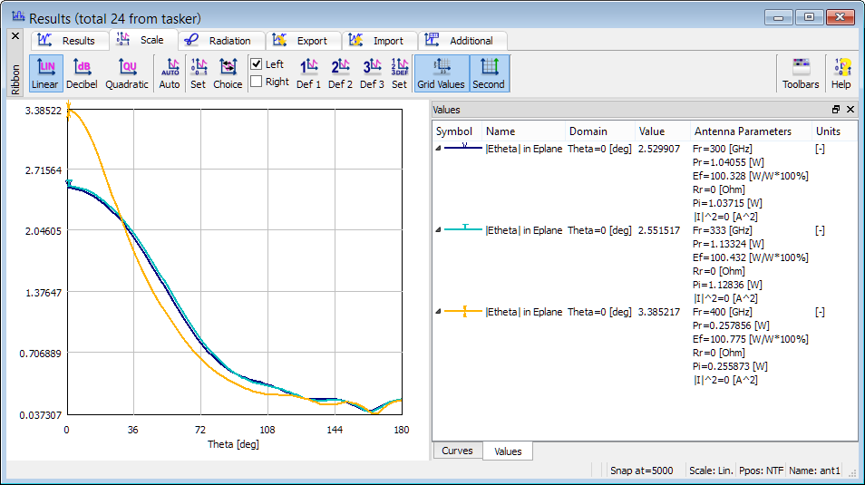
Fig. 2.1-10 The Config dialogue, as used for changing the display from |Etheta| and |Ephi | at the first frequency to |Etheta| at all three frequencies, and the produced display.
We can also watch some combinations of the characteristics. Enter the Config dialogue again, select the |Etheta| curve at the second frequency (position 9 on the list), and press Hide. Now select the remaining two |Etheta| curves, check data1...data2 in the Calculation order field and press the division button (/) within the Calculate new data field. Select the new calculated characteristic and press Show. After setting scale for Y-coordinate to Max=+5, Min=0, Grid Step=1 we obtain the display of Fig. 2.1-11, which shows the |Etheta| characteristics for 300 GHz and 400 GHz, as well as their ratio.
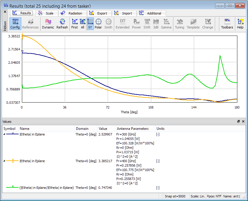
Fig. 2.1-11 The |Etheta| characteristics at 300 GHz and 400 GHz, and their ratio (green).
Finally, note that there are two ways of saving the calculated results on disk:
· Via options available in Export tab of Results window or Setup-Save Results command in main menu. Those options save in one file all the characteristics calculated by the software as defaults for a particular post-processing. In the present example, it will save the amplitudes and phases of Etheta, Ephi, copolar and crosspolar at the three frequencies. However, it will omit all other characteristics, additionally calculated upon the user’s explicit request (via Power option in Results tab (Setup-Switch-Power Balance command in main menu) or Calculate new data operations within the Config dialogue).
· Via Save Sel. operation in the Config dialogue. This command saves only the characteristics previously selected (highlighted) on the Config. list.
Remember that whenever a new project is created, or the meshing of the existing project is changed, the user is advised to take a look at the mesh exported from QW-Editor to QW‑Simulator. Options available in the Mesh tab enable invoking the Test Mesh window of Fig. 2.1-12. The regions filled with different media are displayed in different colours, and also the mesh lines over these regions are marked in different colours, which have been assigned to these media in Project Media dialogue of QW-Editor as Brush and Pen, respectively. To check these assignments, one may go back to QW-Editor, open the Project Media dialogue, and for each medium of interest press the Brush and Pen buttons. In our ant1 example, metal regions are shown in grey with yellow hatch and brownish mesh lines, and air is shown in white with light blue hatch and blue mesh lines. Therefore, what we see in Fig. 2.1-12 is an air-filled space around the metal long-section of the antenna body. The two rows and two columns of metal cells around the air space are added automatically by the software, and should be ignored from the viewpoint of geometry interpretation. They are needed by the software for internal data structure purposes, and do not take an active part in the process wave simulation. Waves travelling over the simulated scenario do not reach these metal boundaries, as they previously encounter the absorbing boundaries marked by blue dashed lines.
The thick blue line passing through the third (from bottom) row of cells marks the magnetic symmetry plane, which here models the axis of rotation. The dashed lines mark, respectively: red – input port, blue – input reference port for return loss extraction, green – NTF box and blue – absorbing walls.
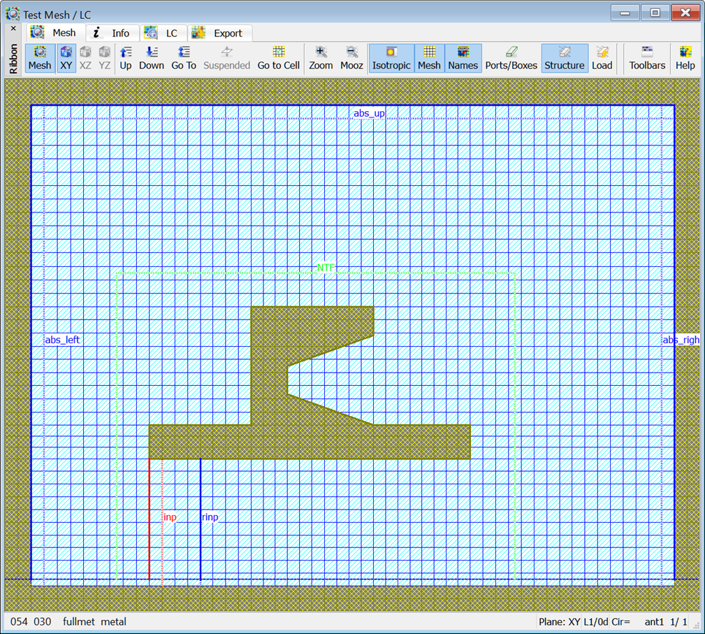
Fig. 2.1-12 Test Mesh window for the ant1 example with Isotropic, Mesh and Structure options.
In Specific aspects of FDTD analysis in V2D it has been stressed that non-axisymmetrical modes can be analysed with either magnetic or electric symmetry model of the axis of rotation. Although somewhat different singularity approximations are applied to different field components in those two cases, both should produce consistent results.
The user wishing to verify the above statement should now: save the results calculated with magnetic symmetry model on disk (Save option of Results window), stop the simulation (Stop option in Run tab), exit QW-Simulator (File-Exit command in main menu), go back to QW-Editor, open the list of elements (Edit-Select Element command in 2D Window), select the element named open_y, press Delete, press Close to exit the list, and press Start button in Simulation tab. Now the Test Mesh window shows the upper display of Fig. 2.1-13. There is no magnetic symmetry plane, and the electric symmetry plane is formed by the upper edge of the second (from bottom) row of auxiliary metal cells.
After 5000 iterations we suspend the analysis and display the radiation pattern results. We use Load option available in Import tab of Results widow and load the previously saved results. In the Config dialogue we perform the following operations:
· press Sel.All and then Hide, to hide all the displayed curves,
· select curves No.1 and No.25, check data2..data1 in the Calculation order field, press ‘–‘ button in the Calculate new data field,
· select curves No.3 and No.27, press ‘–‘ button in the Calculate new data field,
· select curves No.1 and No.49, press ‘/‘ button in the Calculate new data field,
· select curves No.3 and No.50, press ‘/‘ button in the Calculate new data field.
Note that curve No.49 plots absolute difference between amplitudes of Etheta at 300 GHz, calculated with the two axis models. Curve No.50 plots absolute difference between amplitudes of Ephi at 300 GHz, calculated with the two axis models. The lower part of Fig. 2.1-13 shows curves No.51 and No.52, which plot relative discrepancies. We find that the discrepancy is within 1% for angle q<90°. It increases to 6% for q »150°, in which direction the absolute radiated power is very small.
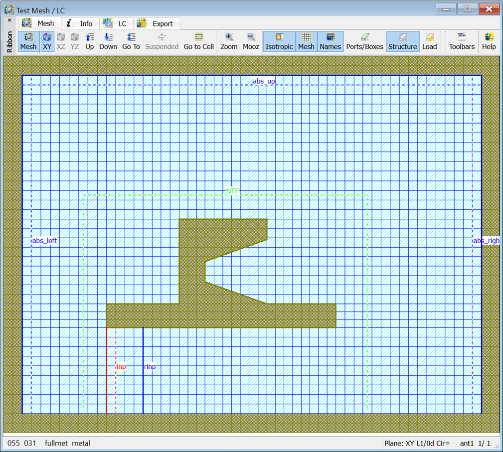

Fig. 2.1-13 Some results of analysis of the modified ant1 example (with PEC model of the axis): Test Mesh window with Isotropic, Mesh and Structure options and relative discrepancy in amplitudes of Etheta (blue) and Ephi (green), with respect to the original ant1.
In a similar way, we can evaluate the influence of meshing on the accuracy. We stop the simulation (Stop option in Run tab), exit the QW-Simulator (File-Exit command in main menu), go back to QW-Editor, re-load the original ant1.pro (File-Open), invoke Mesh Parameters dialogue, introduce 0.02 for Max cell size X, press X to Y, press OK, and press Start button in Simulation tab.
Now the Test Mesh window shows the upper display of Fig. 2.1-14. Since the reduced cell size leads to a reduced time-step, we shall run the analysis for 10000 iterations. Then we repeat the same sequence of operations as in the previous experiment. The lower part of Fig. 2.1-14 shows curves No.51 and No.52, which plot relative discrepancies of Etheta and Ephi at 300 GHz, with respect to the original ant1 project.
Note that the FDTD results with finer mesh are more accurate. Cell size reduction by a factor of two typically reduces the error of analysis by a factor of 2..4. Since the results obtained with cell 0.04 mm differ from those with cell 0.02 mm by less than 1%, we can predict that further cell size reduction would change the results within further 0.25..0.5%. Thus we would estimate the total error introduced by cell 0.04 mm at less than 1.5%.

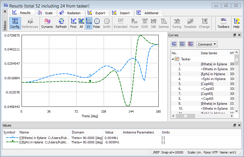
Fig. 2.1-14 Some results of analysis of the modified ant1 example (cell size refined by a factor of 2): Test Mesh window with Isotropic, Mesh and Structure options and relative discrepancy in amplitudes of Etheta (blue) and Ephi (green), with respect to the original ant1.
QW-Simulator offers several ways of field visualisation, which are worth getting acquainted with. However, from the user’s viewpoint, it will be more instructive to watch the fields in the steady-state sinusoidal regime. Therefore, we again stop the simulation (Stop option in Run tab), and exit QW-Simulator (File-Exit command in main menu).
We go back to QW-Editor and load the ant1_sin.pro (File-Open), in which the structure is excited by sinusoidal signal at 300 GHz. Run the simulation by pressing Start button in Simulation tab.
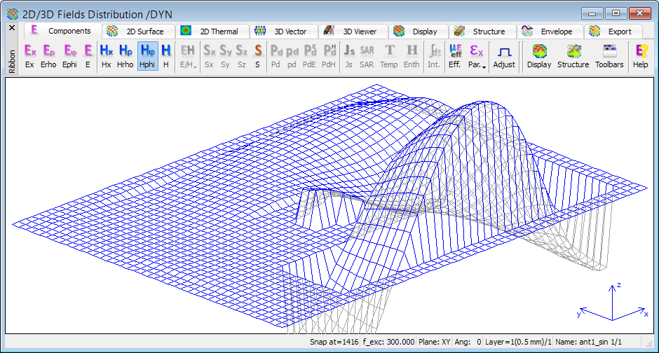
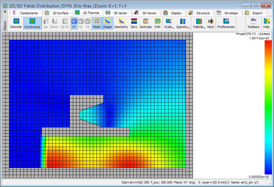
Fig. 2.1-15 Steady-state Hj field at 300 GHz in ant1_sin example: example of instantaneous distribution in the hill-top mode (upper), and envelope in thermal mode with active Isotropic, Mesh and Shape options (lower).
The steady state is reached within 1000 iterations. Fig. 2.1-15 in the upper part shows a snapshot of the azimuthal H-field component at iteration 1416 in the hill-top mode activated with Lines button ![]() from the 2D/3D Fields tab of QW-Simulator. Choosing the Thermal Continuous
from the 2D/3D Fields tab of QW-Simulator. Choosing the Thermal Continuous  option from 2D/3D Fields tab and invoking Hj component distribution opens the 2D/3D Fields Distribution window as shown in the lower part of Fig. 2.1-15, with Shape and Mesh options active. In this window the envelope is built (the type is signalised in the window title bar). The envelope calculation can be activated/deactivated via the options available in Envelope tab of 2D/3D Fields Distribution window.
Let us now change to the azimuthal E-field component using ![]() button in Components tab of 2D/3D Fields Distributionwindow. After the new envelope is built up, we obtain the upper view of Fig. 2.1-16.
button in Components tab of 2D/3D Fields Distributionwindow. After the new envelope is built up, we obtain the upper view of Fig. 2.1-16.
The thermal display permits enhanced resolution of fields in certain regions. We may change the scale to manual using Manual option available under Scale button in 2D Thermal tab of 2D/3D Fields Distribution window, and set Max to 0.02. This leads to the lower display of Fig. 2.1-16.

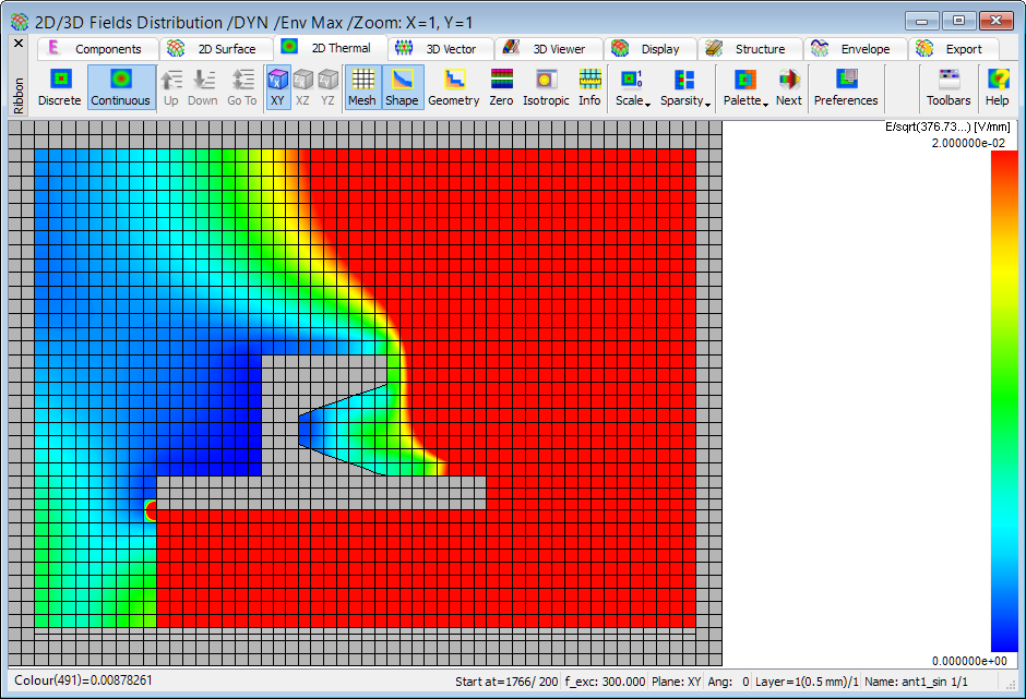
Fig. 2.1-16 Steady-state Ej field at 300 GHz in ant1_sin example: envelope in thermal mode with active Mesh and Shape options. The upper view is in the default Full Auto scale, the lower has been obtained for Manual scale with Max set to 0.02.
Fig. 2.1-17 shows zoomed views. The upper one has been obtained by pressing Z on the keyboard, and using the side and bottom zips to adjust to the corrugation inside. Switching to the Discrete display (in 2D Thermal tab) produces the lower view.

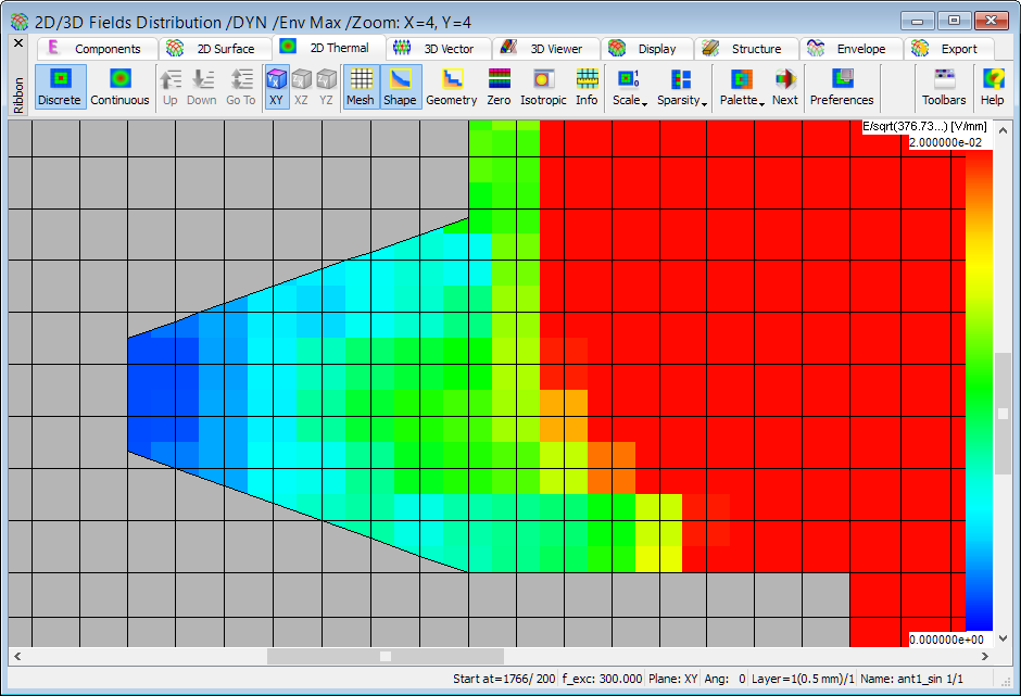
Fig. 2.1-17 Zoomed display of steady-state Ej field envelope at 300 GHz in ant1_sin example: thermal continuous (upper) and thermal discrete (lower).