2.4.1       Heating in circular waveguide with linear polarisation

Microwave heating problems are also, in essence, the problems of solving Maxwell equations in inhomogeneous and lossy space. However, they differ from the previously considered S-parameter and radiation examples in terms of required output. A possibility to watch the field and power patterns is now of primary importance. Additionally, note that we need to know absolute values of fields and power, and not only their relative patterns. In other words, it is not sufficient to find out that we would obtain a hot or a cold spot in a particular scenario; it is equally important to detect the actual maximum temperature (above or below the burning point of our material?) and minimum temperature (above or below microbiological disactivation?).

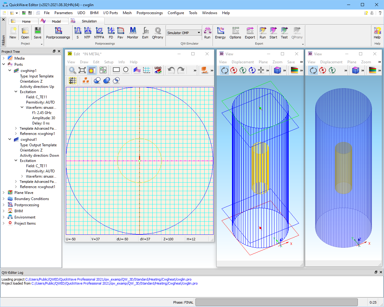
Fig. 2.4.1-1 A view of cwglin.pro in QW-Editor.

As our first problem of this category, let us consider a bread stick heated in a circular waveguide. The bread stick has a radius of 15 mm, length 100 mm, and medium parameters corresponding to the temperature of 20°C (e_r.=4.17, s=0.211 S/m). It is placed centrally in the guide of radius 50 mm. The view of the whole structure, stored in the ..\Heating\Cwgheat\cwglin.pro project, in QW-Editor is presented in Fig. 2.4.1-1.

We shall start our investigation of this example by understanding the displays and settings of QW‑Editor. The users interested directly in the FDTD simulation process and results may now skip one subsection.

Interpreting QW-Editor displays and settings

In Fig. 2.4.1-1 we can see our structure visualised in three windows: 2D Window, 3D Window wireframe view, and 3D Window solid view. We may close the windows and open additional windows by pressing  or  buttons in Home tab, respectively. Note that at least one 2D Window in XY-plane is needed for manual drawing.

Fig. 2.4.1-2 Circuit dialogue of cwglin.pro.

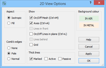
Fig. 2.4.1-3 2D View Options dialogue of 2D window in cwglin.pro.

The 2D Window is marked as QW 2D in its title bar, which also brings an important piece of information: IN METAL. This means that metal is our default medium, or in other words, background medium for this project. All regions meshed but not explicitly filled with any other medium will be filled, by default, with metal. Actually, QW-Editor offers two choices of default media: metal and air. The choice can be made in Circuit dialogue, as shown in Fig. 2.4.1‑2. Here we can verify that our circuit type is 3D, and that our default medium is metal. We may also add a short description. All other settings are irrelevant at this point.

Note that our choice of default medium is also signalled by the background colour of the 2D Window. This can be modified in 2D View Options dialogue, which is shown in Fig. 2.4.1-3. Besides the possibility of changing the background colour, we can see that the FDTD mesh (shown in blue in Fig. 2.4.1-1) and coordinate axes (magenta and brown in Fig. 2.4.1-1) are visible because activated herein. They can be made invisible either here, or via Mesh Parameters and 2D Axes Settings dialogues. We have also chosen isotropic aspect, which means that the display proportions will be fixed irrespectively of the whole 2D Window proportions. Comb’s edges settings are irrelevant because we do not have combined elements in this project. However, it may be useful to know that the elements marked for reproduce operations will be distinguished with thick lines; those selected as active or passive for join operations will not. Checking grid brings up a dotted Cartesian 2D grid, sometimes useful for manual drawing. Lines in plane reduces the contents of the 2D Window to the contours of those elements, which are based at the current level. This level is always signalled in the window status line (Z=100 in Fig. 2.4.1-1).

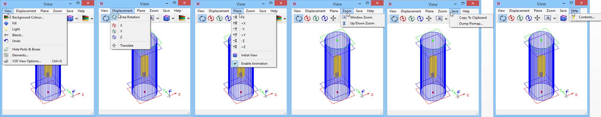
Fig. 2.4.1-4 Options of 3D window in cwglin.pro.

Fig. 2.4.1-5 A modified 3D solid display.

Note that View commands of the 3D Window offer somewhat different selections of settings (Fig. 2.4.1-4), also accessible from the toolbar. In particular, the background colour does not depend on the default medium. Fig. 2.4.1-5 shows 3D solid display with modified background colour, angles and light.

Let us now investigate how our example has been constructed in QW-Editor. Invoking Select Object dialogue (using ) of Fig. 2.4.1-6 (left), we find that only one object named cwgh has been used. Its type is udo, which means that it has been constructed from a parameterised UDO script. When we double-click over this object in the Select Object dialogue (or click once over the object and then over ), QW-Editor opens its script and displays the object header with all its parameters (Fig. 2.4.1-6, right). Thus we learn that the heating device is a circular air-filled waveguide of radius 50 mm and length 300 mm. The bread stick of previously specified parameters is placed centrally (there are no provisions for offset). Note negative answers to questions “Add second source Y/N” and “Add second load Y/N”. This means that we will operate with one source and one load, and – as explained further – with linear vertical polarisation.

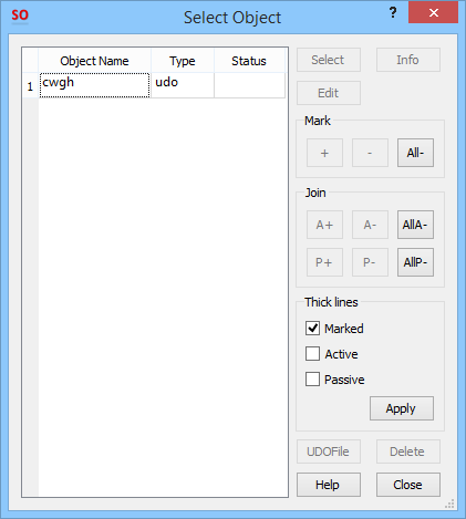
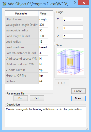
Fig. 2.4.1-6 Select Object dialogue and object header in cwglin.pro.

Note that in the header we can easily modify the available dimensions and media settings. In other words, we can quickly re-construct the considered object without any manual drawing or graphical operations on our side. This is major advantage of using UDO scripts in project building, and we will demonstrate it further in this Section. Other advantages include fast and easy coupling to external optimisers.

Please also note that QW-Editor stores absolute paths to all the *.udo files applied in a particular project in the project’s *.pro file. Thus in cwglin.pro we have the path to:

C:\Program Files\QWED\QW_3D\v____\elib\examples\cwgheat.udo.

 If you have installed the software in other than standard directories, cwgheat.udo will not be found at the location recorded in cwglin.pro, and QW-Editor will issue an error message. In such a case, please open Set UDO’s paths dialogue, click Add Folder, and browse the directories to add an appropriate folder to the list.

As an alternative to looking at the Select Object dialogue and object header, we may verify our project construction through Select Element dialogue (invoked with  button) of Fig. 2.4.1-7 listing all elements and also ports of our project. As we have explained in FDTD Method in QuickWave Software, elements are an intermediate product of the FDTD mesh generation. They appear after all surfaces have been faceted. Therefore each element has the shape of a prism, based at a particular Z level, of a particular Height along the Z-axis, and filled with a particular Medium - as indicated in Fig. 2.4.1-7. In our case, geometry variation along the Z-axis is very simple and therefore the list of elements is very short: there are two faceted cylinders named cwghwg and cwghld. Their faceting has been determined by the number of sectors set in the object header (right in Fig. 2.4.1-6). Clicking over cwghwg on the Select Element list and then over , we obtain Element Details shown on the right of Fig. 2.4.1-7, and confirming that the circular base has been approximated by a polygon of 64 segments named W0..W63.

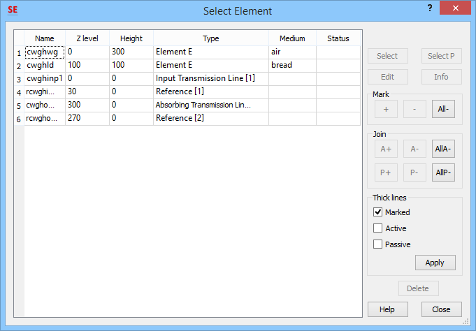
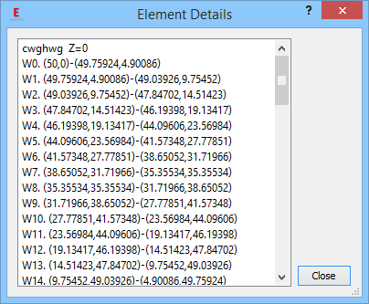
Fig. 2.4.1-7 Select Element dialogue in cwglin.pro.

The Select Element list also indicates Type of each item. For ports this is self-explaining. For elements, it signals their mesh-snapping properties. In particular, Element E in Fig. 2.4.1-7 means that both cwghwg and cwghld will always force electric mesh snapping planes (i.e., FDTD mesh levels where the tangential electric fields are defined) at their bottom and cover along the Z-axis.

Operating on the Select Element list is sometimes convenient for manual project modification. We will demonstrate this later in the present Section.

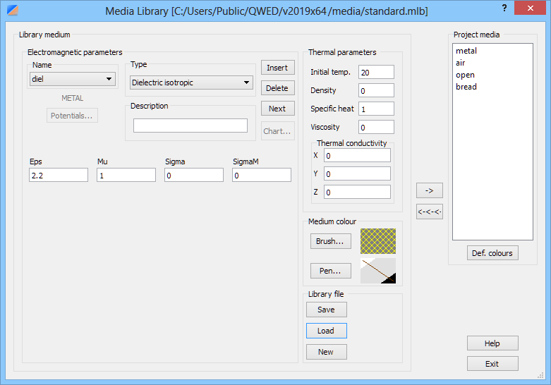
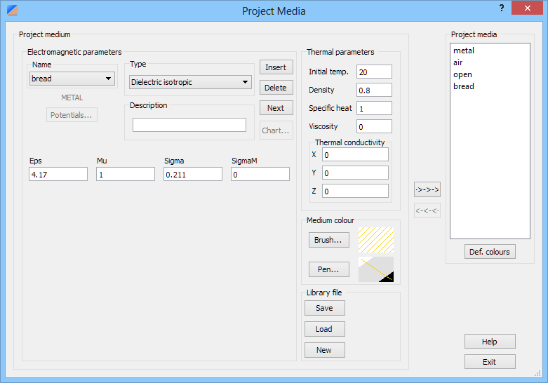
Fig. 2.4.1-8 Media library and Project Media dialogues in cwglin.pro.

Now we may wish to verify if physical parameters of the media named air and bread (Fig. 2.4.1-6, Fig. 2.4.1-7) have been correctly set. We invoke Project Media dialogue of the QW‑Editor. The right hand side shows the current Project media and by default they are shown also in the left hand side.

Note that only the left hand side allows inserting (Insert button) new media, deleting (Delete button) existing media or modifying their parameters via dialogue boxes. We can also control the display of elements filled with a particular medium via Pen and Brush buttons.

There are several ways of dealing with media in QW-Editor:

·       Acting on the library level: We can create our own library or a system of libraries. We use: New button to start up a new library file (the Project Media dialogue changes to Media Library dialogue as in Fig. 2.4.1-8 (upper)); Load button to load an existing library file; Insert button to add a new medium to the current library; dialogue boxes to modify the current medium; Next button to see the next medium in the current library or Name list:  to select a medium from this library; Save button to save the current library on disk. Picking up a medium from the current library to the current project: This is accomplished via  button.

·        Acting on the project level, which is most typical way of managing the media. The actions are performed in Project Media dialogue (Fig. 2.4.1-8 (lower)): Project Media dialogue is typicaly in the edit mode. We can now deal with our project media using the same buttons as previously for the library media, the only difference being that QW-Editor will not allow us to delete a medium already assigned to some element(s) in the project. We then store the new media settings via  command. Note that a new project started in QW-Editor via the File-New command inherits the media from the previous project. For more details on media parameters and media libraries, please refer to Media and Libraries of QW-Editor, respectively.

Here let us note that the first way above is recommended if you deal with many different media, in various applications and technologies. The second way can be convenient if the scope of the considered media is limited and their parameters do not change with application and/or technology; we will proceed this way here.

Let us now look at the parameters of bread in the Project Media dialogue of Fig. 2.4.1-8. Regarding bread, we can see that:

·       It is Dielectric isotropic.

·       Bread’s relative permittivity Eps and relative permeability Mu are set to 4.17 and 1, respectively.

·       Bread does have electric volume losses. Sigma field allows us to define electric conductivity in [S/m]. Note that 0.211 S/m at 2.45 GHz corresponds to e_r’”=0.211/(2p*2.45/(36p))=1.55 and, in view of the previously defined  e_r’=4.17, tand=0.37.

·       Magnetic volume losses, defined in SigmaM field, are zero.

·       Density is set at 0.8g/cm³. This will allow SAR calculations in QW-Simulator. Other Thermal parameters: Specific heat and Initial temperature will be used only if QW-3D operates jointly with the optional QW-BHM module.

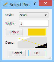
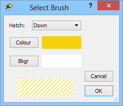
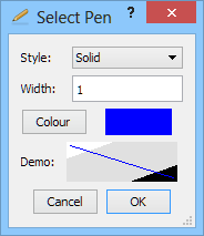
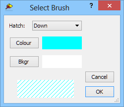
Fig. 2.4.1-9 Pen and Brush dialogues for bread and air in cwglin.pro.

·       We can control the display of bread-filled regions in QW-3D. In Project Media dialogue, click over Pen button and you will see a dialogue as on the left of Fig. 2.4.1-9. Here we can set the colour for displaying bread regions in QW-Editor 2D and 3D Windows; line width and line style appear directly in 2D Window.

·       We can control the display of bread in Test Mesh window of QW-Simulator. Brush settings apply to bread-filled regions; Pen settings apply to mesh lines over these regions.

Concluding our discussion of media settings, let us choose air medium from the Name list and take a look at its parameters as shown in Fig. 2.4.1-10. As expected, it is lossless, dielectric isotropic with Eps=1 and Mu=1. Moreover, its density is not set, so it will not take part in SAR calculations or in temperature / enthalpy calculations with QW-BHM module.

Fig. 2.4.1-10 Air parameters in cwglin.pro.

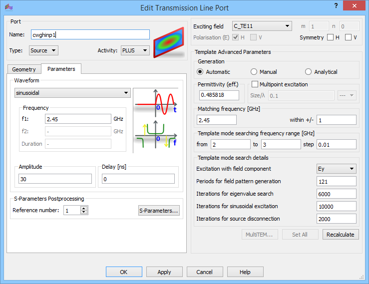
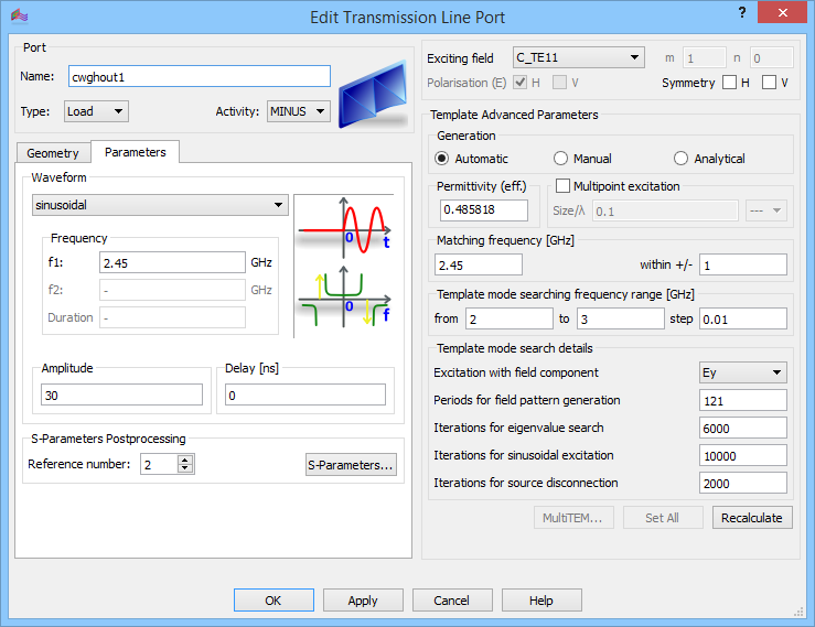
Fig. 2.4.1-11 Parameters of input (upper) and output (lower) ports in cwglin.pro.

Now, we will investigate the input and output port settings. Open Transmission Line Ports dialogue to invoke Edit Transmission Line Port dialogues for source and load port (Fig. 2.4.1-11).

Both ports are bound to the circular waveguide fundamental mode, and therefore in both cases we have Exciting field: C_TE11. The Excitation Waveform is set to sinusoidal at f1: 2.45 GHz and sketched graphically together with its frequency-domain spectrum. The spectrum is not perfectly delta-shaped because the excitation starts at a particular time instant and lasts for a finite time. The Amplitude is set to 30, which means that the source of 900 W time-maximum available power will be applied.

Although this setting has been made for both ports, note that only the port marked as Source will be excited. The port marked as Load is forced to passive state and acts as an absorbing load. Thus in our example, Excitation Waveform is irrelevant for cwghout. Let us note that the reason why we allow for setting Excitation Waveforms for Loads is related to the Smn postprocessing addressed in Advanced S-parameter problems for waveguide-to-coax example and further in S-Parameters. In Smn operation, QW-3D software applies excitation from each of the ports (either consecutively or in parallel), and assembles all the results into a complete S-matrix.

Several of our projects previously considered in S-parameter extraction problems and Radiation Problems have been concerned with rectangular waveguide technology. In the case of a rectangular waveguide, modal indices unambiguously determine wave polarisation. For example, in our Waveguide-to-coax transition, the choice of R_TE10 mode (Fig. 2.2.1-6) has been bound to the vertical E_z field. A distinctive feature of a circular waveguide resides in its axial symmetry. The C_TE11 mode in our example can be induces and propagate with any orientation of the E-field in the XY-plane. Now we shall use a default polarisation applied by the software, which is a vertical polarisation associated with the dominant E_y field. It is signalled in the 2D Window of Fig. 2.4.1-1 by a small red vertical dipole in the port centre; we can also verify this in Edit Transmission Line Port dialogue as in Fig. 2.4.1-11 where we see “Excitation with Ey field component”.

One more important box in the Edit Transmission Line Port dialogue is Permittivity (eff.). It will be used at the load for optimising the absorption of the considered mode at the considered frequency, and at both ports for generating the templates. The meaning of effective permittivity has been discussed in detail in First insight template generation. Here let us only note that our TE11 mode propagates in the defined circular waveguide at 2.45 GHz with propagation constant 0.036 mm^-1; with the same propagation constant a plane wave in free space propagates at the same frequency 2.45 GHz if the space is filled with a medium of relative permittivity 0.486.

As a final step before launching the FDTD simulation, let us verify the mesh settings via the Mesh Parameters dialogue, which for this example is as shown in  Fig. 2.4.1-13. First of all, it instructs the software that Max cell size should not exceed 3 mm in any direction. Note that at 2.45 GHz we have a wavelength of 122 mm in air, and 60 mm in bread. Thus the selected discretisation in our project resolves the wavelength into at least 20 cells, which brings the inherent FDTD dispersion errors below 0.25%. It also accurately resolves the smallest dimension – bread radius – into 10 cells, which similarly reduces the error of geometry approximation.

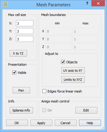
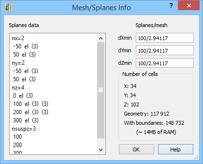
Fig. 2.4.1-13 Mesh Parameters dialogue and its Mesh/Splanes Info part in cwglin.pro.

Discretisation is always a trade-off between accuracy and computer resources.  button invokes Mesh/Splanes Info window, where the user can check that the created Number of cells is 117912, while QW-Simulator will consider 148732 to additionally allow for boundary effects. This requires only 14 MB of RAM, and as we shall see, the analysis will be rapid. In other words, in this simple project we do not need to optimise the meshing to save on memory and CPU time. In more complicated projects, as we shall see in further Sections, we can for example apply finer meshing within the regions of faster field variation (higher permittivity, complicated boundaries, etc), and coarser meshing elsewhere. This is achieved with the use of mesh snapping planes (also called special planes of Splanes), listed on the left hand side of Mesh/Splanes Info dialogue. In our case, the only Splanes are those enforced by the objects boundaries. The dXmin, dYmin, dZmin fields of the Mesh/Splanes Info dialogue show the minimum distance between two consecutive mesh snapping planes along each direction, and the resulting minimum FDTD cell size. Since 100 is not commensurate with the max cell size of 3 mm, somewhat smaller cells of approximately 2.94 mm have been generated.

Since the Objects box is checked in Fig. 2.4.1-13, the whole defined structure has been meshed. An alternative would be to restrict the FDTD simulation to the region confided within Mesh boundaries, taking advantage of structure symmetry. We shall consider this possibility later.

Now we should feel confident about current project settings and we can start its analysis by pressing  in Simulation tab of QW-Editor.

Running QW-Simulator and monitoring the fields

QW-Simulator has been automatically started and its main window has appeared on the screen. The title bar includes the available options, version number and date, hardware key type, and our project name. Below the main toolbar we have a Simulator Log window, which monitors the consecutive operations performed by the software (Attention: if you do not see the Simulator Log window at all, it has been closed by previous users of your QW-3D installation; please restore it via View-Simulator Log command). The two sections starting with Cell Descriptors Reading… and terminating with Template calculations completed and saved correspond to preprocessing operations, when QW-Simulator solves an eigenvalue problem in the ports cross-section, determines the modal field templates, and saves them on disk. The third action of Cell Descriptors Reading… is for the whole 3D structure. A few flushes through the progress bar at the bottom of Simulator Log show the progress of transforming the geometrical data into the so called LC matrices, later used by the software as coefficients for field updating. Finally the progress bar shows “FDTD preprocessing done” message and the iteration counter in the status line of the main window indicates the progress of the 3D analysis.

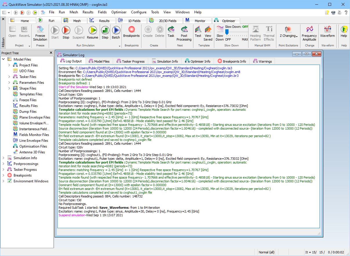
Fig. 2.4.1-14 Main window of QW-Simulator: with Simulator Log and status line after 15 iterations.

To catch the displays at an early stage of the simulation, we have pressed the Suspend button  from Run tab of QW-Simulator window, (thus Simulator Log of Fig. 2.4.1-14 terminates with Suspend simulation). After pressing Fields  button (in 2D/3D Fields tab of QW-Simulator) 2D/3D Fields Distribution window is opended and we can see the pattern of the longitudinal H-field of the wave entering the guide, in the central long-section of the guide. Note that the settings for this window have been read by QW-Simulator from cwglin.en8 file delivered on the installation DVD. This file is modified by the software at every Stop () or Exit (of the main window) operation. Therefore if your installation has previously been used and cwglin has been simulated, cwglin.en8 may have been modified, and you will see a different display.

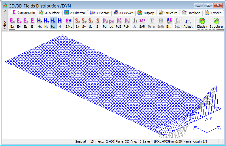
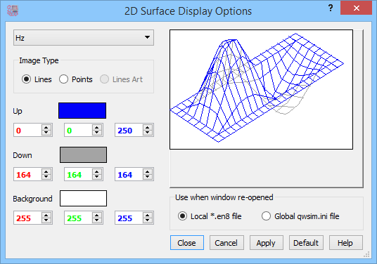
Fig. 2.4.1-15 2D/3D Fields Distribution window of QW-Simulator after 15 iterations (left) and 2D Surface Display Options for this display (right).

You can restore the display of Fig. 2.4.1-15 with the available buttons and commands:

·       press  button in Components tab,

·       press  button in 2D Surface tab (you should see Plane: XZ in status bar),

·       press  or  button in 2D Surface tab until you see Layer:19/38 in status bar; alternatively, press  button and set 19 in the Go to.. dialogue,

·       press  button in 2D Surface tab to adjust the scale of display to the window dimensions,

·       press D on the keyboard until you see /DYN in title bar,

·       if your display is not of the Surface type as in Fig. 2.4.1-15, but instead looks like a colour map (please look at Fig. 2.4.1-18 to see the difference), then press press  button in 2D Surface tab of 2D/3D Fields Distribution window.

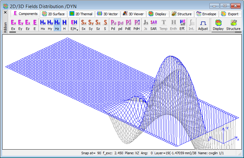
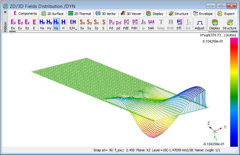
Fig. 2.4.1-16 2D/3D Fields Distribution window of QW-Simulator after 90 iterations.

Note that the main window commands have been supplemented with a Setup group for the 2D/3D Fields Distribution window. All the above buttons are shortcuts to Setup commands. These commands are also accessible from the floating menu, available upon right mouse button click over the window, and from keyboard entries.

After performing all the above operations, your display may differ from that of Fig. 2.4.1-15 in terms of colours, if previous users have changed the display options. To modify the colours, open 2D Surface Display Options shown in the right part of Fig. 2.4.1‑15.

Pressing Resume  button (in Run tab) would now resume the FDTD simulation and we would quickly reach the steady state. However, in some cases we may wish to slowly investigate the transient phenomena. Then it may be convenient to move step-by-step, by pressing  button. For example, after 90 iterations, we can clearly see the disturbance of the wave impinging at the dielectric cylinder (Fig. 2.4.1-16). The upper display in Fig. 2.4.1-16 is in Lines mode ( button in 2D Surface tab); the lower one is in Art mode ( button in 2D Surface tab).

We now press  button and the analysis proceeds automatically, with dynamic monitoring of the longitudinal H-field. Note that dynamic displays slow down the FDTD simulation. To restore its speed, we can:

·       press D on the keyboard to switch the dynamic display off; the /DYN flag in the 2D/3D Fields Distribution window will disappear;

·       invoke Refresh Settings dialogue; in the dialogue of Fig. 2.4.1-17 we may instruct the software to refresh display periodically but less frequently than at each iteration;

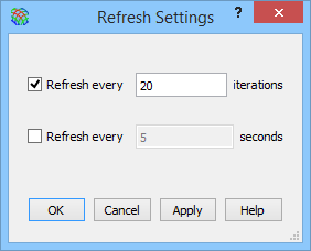
Fig. 2.4.1-17 Refresh Settings dialogue window of QW-Simulator.

After a few hundred iterations the steady state is reached. It is now instructive to create the field envelope. While in /DYN mode, activate the envelope maximum calculation by pressing  button in Envelope tab of 2D/3D Fields Distribution window or by pressing E on the keyboard. By definition, we must wait for at least one period to produce the envelope; please also note that it may visibly vary over many periods if the discretisation is coarse and the period is not commensurate with the time step. The views of Fig. 2.4.1‑18 have been snapped when the display has stabilised, starting at iteration 700 and lasting for 300 iterations, as indicated in the status line (start at: 700 / 300).

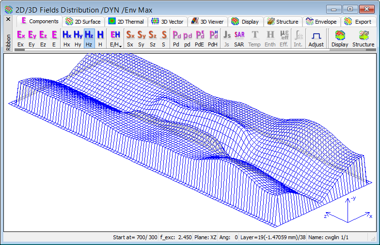
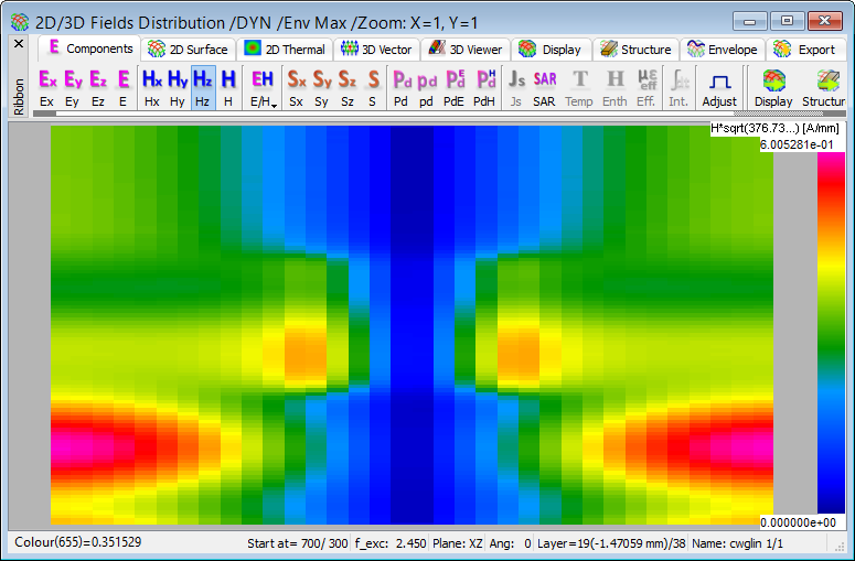
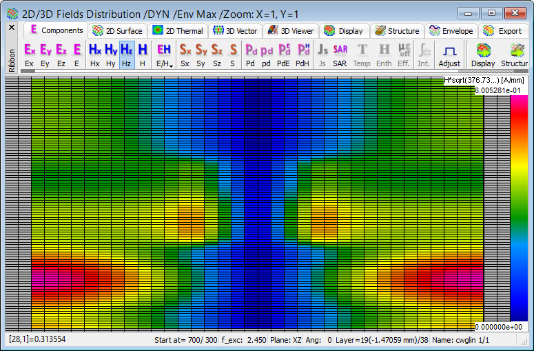
Fig. 2.4.1-18 Longitudinal magnetic field envelope constructed between 700 and 1000 iteration, shown in 2D Surface (upper left), 2D Thermal continuous (upper right), 2D Thermal discrete (lower left) and 2D Thermal continuous with mesh (lower right) mode.

At this point, let us express the duration of one time step in physical units. First of all, we can check it in Simulation Info tab of Simulator Log window. We scroll through the window contents until we find: “Time dt: 0.00490534 [ns]”. We can also justify that this value comes from the applied meshing and FDTD stability criterion. As we have seen in Fig. 2.4.1-13, the smallest cell size is approximately 2.94 mm, which makes 41.6 cells per free space wavelength at 2.45 GHz. The stability criterion in QW-3D dictates that the time resolution must be twice finer than the free-space resolution, so at 2.45 GHz we operate with 83.2 iterations per period. This leads to the time step being equal to 0.0049 ns.

Let us come back to the envelopes of Fig. 2.4.1-18. We can switch from 2D Surface to 2D Thermal display by choosing Distrete or Continuous mode in 2D Thermal tab of 2D/3D Fields Distribution window. By pressing  button for the second time, you should obtain 2D Thermal Continuous view as in the upper right of Fig. 2.4.1-18. You can switch between the two thermal modes by pressing appropriate button (Discrete or Continuous) in the 2D Thermal tab. Actually, the thermal mode allows many more options available in the 2D Thermal tab. In particular, we can switch on and off the display of FDTD mesh lines (see lower right of Fig. 2.4.1-18) with  button).

An important advantage of thermal displays is that we can directly read the physical field values. For example, in the lower right display of Fig. 2.4.1-18 the status bar shows: [28,1]=0.0314. The two integers in bracket show the cursor position counted in cells, in X - and Z-direction. The time-maximum value of H_z in this cell is 0.0314/sqrt(120p) A/m. We will come back to practical applications of this feature later.

Note that 2D Thermal display fills the whole 2D/3D Fields Distribution window. Fig. 2.4.1-19 shows how we can modify this window so as to resemble natural proportions of the structure (which are 3:1 in the central XZ-plane). The left envelope has been obtained analogously as in Fig. 2.4.1-18. Then it has been changed to the display on the right by pressing  button in 2D Thermal tab, which switches on isotropic view of the display..

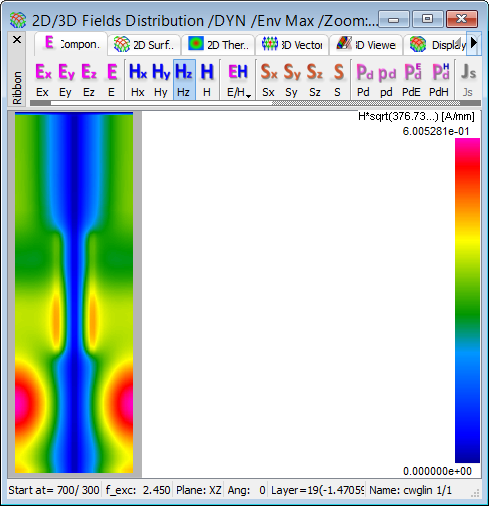
Fig. 2.4.1-19 Longitudinal magnetic field envelope constructed between 700 and 1000 iteration, shown in thermal continuous mode; left – window of equal dimensions; right – window with isotropic view.

So far we have been looking at the longitudinal H-field to get acquainted with QW-Simulator displays. Let us now look at the quantity of major interest in microwave power applications – dissipated power.

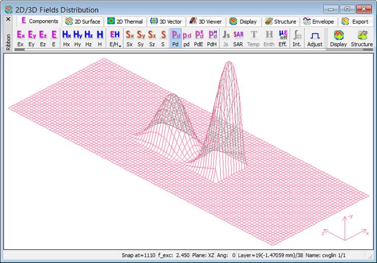
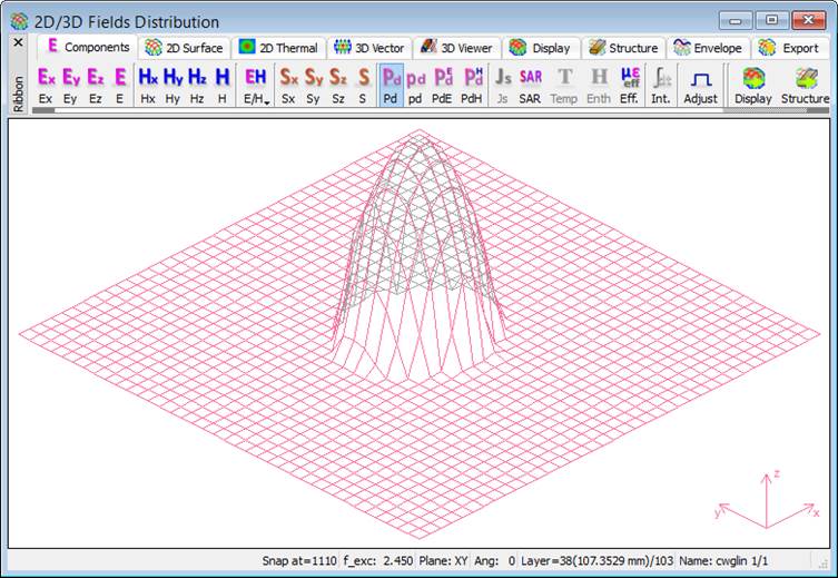
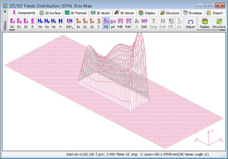
Fig. 2.4.1-20 Dissipated power distribution: instantaneous at iteration 1110 (upper) and envelope (lower), in central XZ-plane (left) and in XY-plane at the lower end of the load (right).

Press  button in 2D/3D Fields tab twice and the 2D/3D Fields Distribution windows as in upper left and upper right of Fig. 2.4.1-20 appear respectively. The windows show the dissipated power pattern. The upper right display in Fig. 2.4.1-20 shows power distribution in the cross-section of the load.

Now to synchronise both windows, press  button, set both windows to the dynamic mode (signalled by /DYN in title bar and produced by pressing  button in Display tab of 2D/3D Fields Distribution window or keyboard D), and then to envelope mode (signalled by /ENV and produced by pressing  button in Envelope tab of 2D/3D Fields Distribution window or by pressing E on the keyboard.). Press   button in Run tab of QW-Simulator. After a few periods you will see the envelopes as in the lower part of Fig. 2.4.1-20.

We observe nonuniformity of power distribution, in longitudinal as well as cross-sectional patterns. QW-3D allows us to investigate its causes and to quickly verify various concepts for improving the system performance. First of all, the longitudinal nonuniformity naturally results from power dissipation as the wave propagates along the load, but also from wave reflections at the end of the load. Cross-sectional nonuniformity results from the modal field pattern.

Before further investigating the nonuniformity of power distribution and proposing system improvements, let us look at other possibilities of visualisation of heating patterns in QW-3D. The following physical quantities are relevant and available for monitoring:

 – power dissipated per cell [W]

 – dissipated power density [W/mm³]

 – specific absorption rate [W/kg]

 – total electric field [V/mm]

The envelopes of these four quantities are collated in Fig. 2.4.1-21 and in Fig. 2.4.1-22. The displays of the above quantities are available after consecutive presses of  button. The displays are in dynamic mode thus they may slow down the simulation. Before calculating the envelope for those quantities it is recommended to disable the dynamic mode in previously opened windows. The calculation of envelope maximum can be enabled with Max button from Envelope tab of 2D/3D Fields Distribution window.

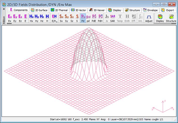
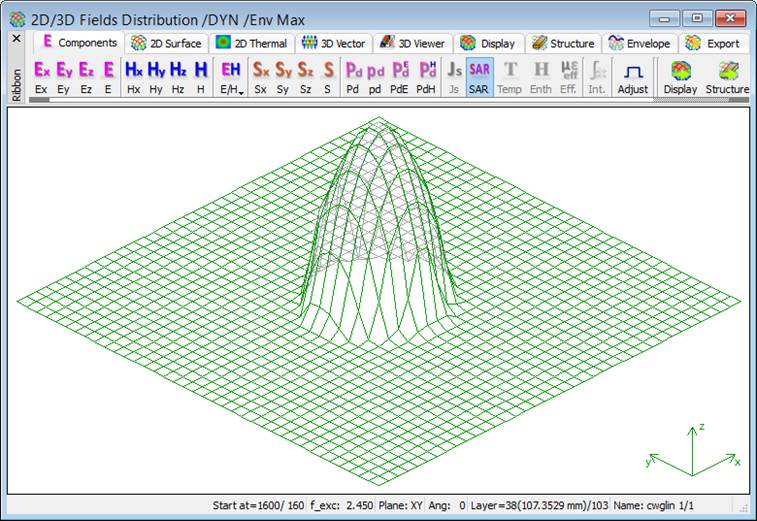
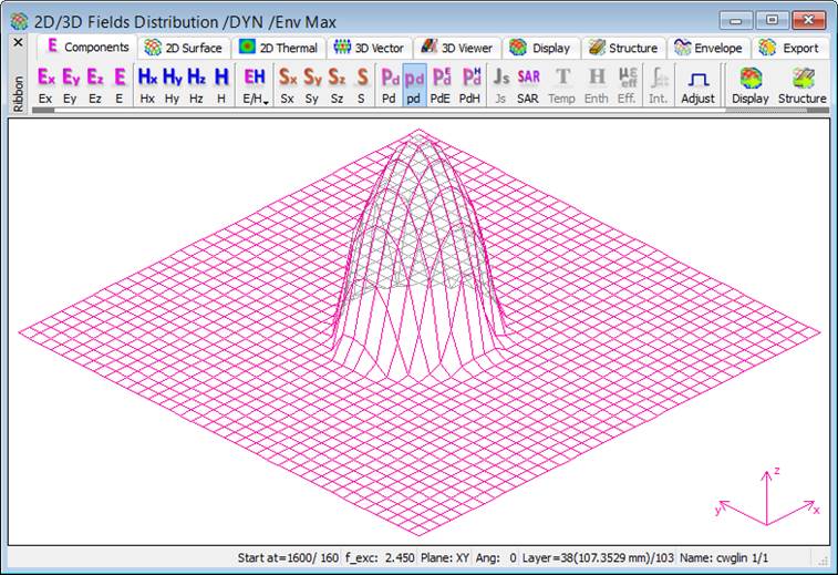
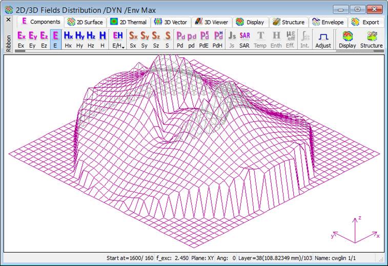
Fig. 2.4.1-21 2D Surface display of envelopes constructed across the load between 1600 and 1760 iteration: dissipated power (upper left), dissipated power density (lower left), SAR (upper right), and total electric field (lower right).

2D Surface displays of Fig. 2.4.1-21 are switched to 2D Thermal of Fig. 2.4.1-22 by pressing  button in 2D Thermal tab of 2D/3D Fields Distribution window (in 2D Thermal displays Isotropic and Shape options are active).

 In Fig. 2.4.1-21 the displays of dissipated power per cell, dissipated power density and SAR look identical as they should be (see Dissipated power and dissipated power density and SAR). Note that the scaling factor between dissipated power per cell and dissipated power density is cell volume, and in this project uniform meshing has been applied. The scaling factor between dissipated power density and SAR is material density, and in this project the whole heated load is made of one material, bread, of homogeneous and temperature-invariant density set as 0.8 g/cm³. Since the  buttons have been pressed, all the displays occupy their full windows, and differ only in colour.

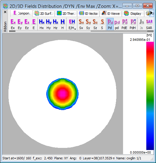
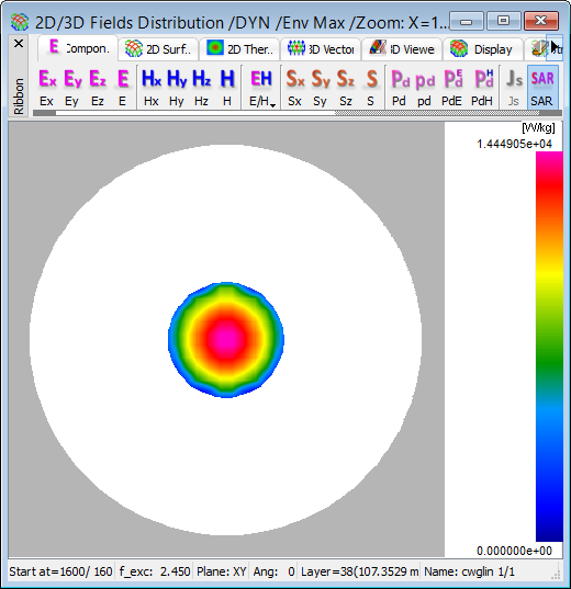
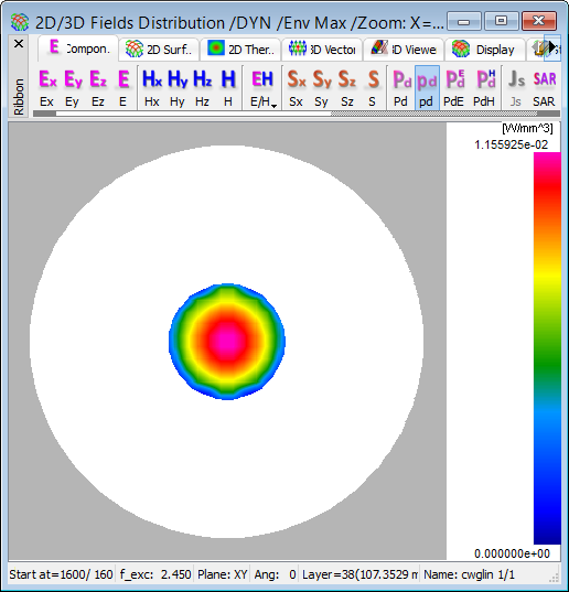
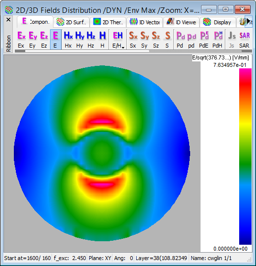
Fig. 2.4.1-22 2D Thermal continuous display of the envelopes of Fig. 2.4.1-21 constructed across the load between 1600 and 1760 iteration: dissipated power (upper left), dissipated power density (lower left), SAR (upper right), and total electric field (lower right).

We can investigate the preservation of power and SAR pattern shapes in more details through their thermal displays of Fig. 2.4.1-22. Power per cell and power density remain indistinguishable, even in Fig. 2.4.1-23 where we have switched to the more revealing Discrete displays, zoomed them at the load (by locating the mouse pointer at the centre and pressing Z on the keyboard), and additionally added the display of FDTD mesh ( button). Regarding SAR, it remains practically indistinguishable from the two power patterns.

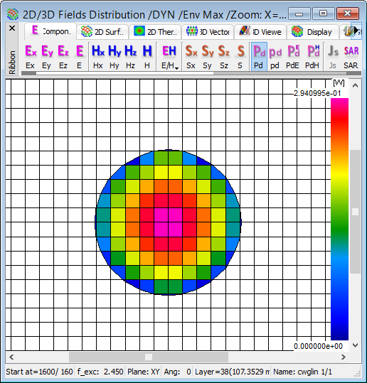
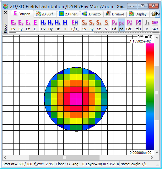
Fig. 2.4.1-23 2D Thermal Discrete display of the power envelops of Fig. 2.4.1-21.

Finally, let us comment on the total electric field displays as in the bottom right corner of Fig. 2.4.1-20, Fig. 2.4.1-21. It differs from the displays of the other three quantities. Naturally, it assumes nonzero values also in air. As we can also expect, considering that the dominant electric field is E_y, there is a strong discontinuity at the boundary between bread and air along the Y-axis. However, what appears in contradiction to the previous conclusions based on the power and SAR patterns, is that the total field pattern indicates rather uniform heating within the load. This is mainly a visual illusion caused by the default Full Auto colour scale in all the displays. The colour palette from navy blue to magenta effectively spans a much wider scale in the case of total electric field (from zero at the waveguide wall where the dominant E_y vanishes - to maxima in air, at the boundary with bread where the dominant E_y experiences a “jump”) than in the case of power and SAR. In other words, what the full colour palette covers over the bread region for power and SAR is subdued to its yellowish-greenish part for total field.

For clearer exemplification, let us invoke instantaneous patterns of total electric field and dissipated power density, at the same iteration 3600, in the same layer 38, discrete thermal mode, with Shape and Mesh options on, and double-zoom around the centre. These are the left and right displays of Fig. 2.4.1-24. Moving the cursor over the left display, we read (in the window status bar) that the total electric field value in the centre is approximately 0.318 (in units to be explained) while about 5 cells away to the left (i.e., at the media boundary) it drops to 0.213. We now invoke choose Manual option from Scale drop down list in 2D Thermal tab and in the Scaling dialogue as seen in the central part of Fig. 2.4.1-24 we set Max=0.318, Min=0.213. The central display of Fig. 2.4.1‑24 results and now looks in reasonable proportion to the power density display on the right. However, we cannot expect perfect resemblance between the power and total electric field patterns. First of all, power variation is quadratic with respect to the total electric field. Secondly, these two quantities are obtained by different averaging schemes, from electric field components calculated at different points in space.

In this example the load cross-section is resolved roughly into just five cells per radius, so the effect of quadratic power variation is not visible. In fact, it is dominated and hidden by the different spatial averaging schemes applied. Note that averaging is essential in FDTD since the field components are staggered on the FDTD mesh, as discussed in FDTD method in QuickWave Software. Moreover, in QW-3D two different averaging schemes are applied to the power and total field patterns. This is indicated by different centering of their displays - please compare the four magenta cells around the load centre in power display versus one offset centred magenta cell in the field display in Fig. 2.4.1-24. Fig. 2.4.1-24 explains which field components are taken for dissipated power calculation, and which for the total field.

The use of two different averaging schemes provides additional information to the user. For example, a discrepancy between the dissipated power density calculated in a particular cell and that extracted from the total electric fields centred at this cell corners (and, of course, multiplied by medium conductivity) can be considered as an error bound for the extraction microwave-heating quantities from FDTD field analysis.

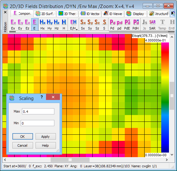
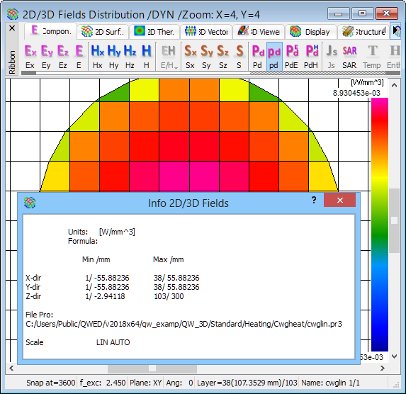
Fig. 2.4.1-24 2D Thermal Discrete display of instantaneous  patterns at iteration 3600: total electric field in automatic scale with Geometry Info (wpper), total electric field in manual scale, with Scaling dialogue open (centre), and dissipated power density with Info 2D/3D Fields (lower).

Finally, let us pay attention to small dialogues and information boxes, popped up upon the field displays of Fig. 2.4.1-24. They can be invoked through Setup command, or right mouse button click over the window, or appropriate keyboard shortcuts. Starting from the right, Info 2D/3D Fields recalls the units in which QW-3D calculates the display quantity; for dissipated power density, these are shown to be [W/mm³]. Scaling dialogue shows the current scale limits and allows changing them. XYZ mm is invoked by Geometry Info option and shows current location of the cursor as well as cell dimensions and volume of the cell it points to. We have requested our project to be been meshed uniformly. However, moving the cursor we can see that cell volumes vary between 22.449659 mm³ and 22.450008 m³, that is, at the 10^-5 level. These results from QW-Editor exporting mesh lines locations in the format of six significant digits. Such discrepancies are irrelevant in all practical cases, as long as reasonable units are used in project drawing. For more information on this subject please refer to Units.